| Accept H0 | Reject H0 | |
|---|---|---|
| H0 is true | True positive | False negative |
| H1 is true | False positive | True negative |
Power and sample size
Computing power and sample size are common tasks in study design. This chapter will walk you through power analysis for network studies. First, we will start with some preliminaries regarding error types and statistical power.
Error types
One of the most important tables we’ll see around is the contingency table of accept/reject the null hypothesis conditional on the true state:
A better way, more statistically accurate version of this table would be
| Accept H0 | Reject H0 | |
|---|---|---|
| H0 is true | Correct inference | Type I error |
| H1 is true | Type II error | Correct Inference |
With \Pr{(\text{Type I error})} = \alpha and \Pr{(\text{Type II error})} = \beta. This way, power can be defined as the probability of rejecting the null given the alternative is true, \Pr{(\text{Reject H0}|\text{H1 is true})} = 1-\beta.
Example 1: Sample size for a proportion
Let’s imagine we are preparing a study in which we would like to estimate the proportion of individuals with a given status. Formally, we then say that the variable Y\sim\text{Bernoulli}(p). To do so, we will need to survey n individuals and estimate such a number by taking the sample average. Furthermore, we hypothesize that under the null the proportion is H_0: p = p_0.
The key here is to think about a simple rejection rule. Again, power is the probability of rejecting the null given that the alternative is true. So, to write down the equation, we need to think about acceptance and rejection regions. Let \hat p be our estimate for the population parameter, furthermore, \hat p = n^{-1}\sum_i y_i. Our test statistic can be–and will be, most of the cases–standardized to leverage the law of large numbers; under the null, we write the following:
\begin{align*} \mathbb{E}(\hat p) & = p_0 \\ \mathbf{Var}(\hat p) & = \sqrt{p_0(1-p_0)/n} \end{align*}
Therefore, the statistic:
\begin{equation*} \frac{\hat p - p_0}{\sqrt{p_0(1-p_0)/n}} = \frac{\sqrt{n}(\hat p - p_0)}{\sqrt{p_0(1-p_0)}} \sim \text{N}(0, 1) \end{equation*}
Since the statistic is normally distributed, we can then say when we will reject the null. For this case, that depends on the critical value, which most of the time is defined in terms of the type I error rate. Formally, we reject the null if
\begin{equation*} \frac{\sqrt{n}(\hat p - p_0)}{\sqrt{p_0(1-p_0)}} > Z_{1-\alpha/2} \end{equation*}
This is equivalent to saying that the test statistic fell into the rejection region. With this in hand, we can now write out the equation that we will be using for calculating the sample size. Going back to the definition of power:
\begin{align*} \Pr{(\text{Reject H0}|\text{H1 is true})} & = 1-\beta \\ \Pr{\left(\frac{\sqrt{n}(\hat p - p_0)}{\sqrt{p_0(1-p_0)}} > Z_{1-\alpha/2}\right.\left|\vphantom{\frac{1}{2}}p = p_1\right)} & = 1 - \beta \end{align*}
Observe that we cannot compute the power for all p\neq p_0; instead, we look at a given parameter value. A good idea is to start from one previously known or identified in other studies. The key idea here is to be able to manipulate the argument of the probability to turn it into a known distribution, for example, the normal distribution:
For a given Type I of 0.05 and power of 0.8, the required sample size can be computed as follows:
\begin{align*} 1 - \beta & = \Pr{\left(\frac{\sqrt{n}(\hat p - p_0)}{\sqrt{p_0(1-p_0)}} > Z_{1-\alpha/2}\right.\left|\vphantom{\frac{1}{2}}p = p_1\right)} \\ & = \Pr{\left(\frac{\sqrt{n}(\hat p - p_0)}{\sqrt{p_0(1-p_0)}} < Z_{\alpha/2}\right.\left|\vphantom{\frac{1}{2}}p = p_1\right)} \\ & = \Pr{\left(\frac{\sqrt{n}(\hat p - p_0)}{\sqrt{p_1(1-p_1)}} < \frac{Z_{\alpha/2}\sqrt{p_0(1-p_0)}}{\sqrt{p_1(1-p_1)}}\right.\left|\vphantom{\frac{1}{2}}p = p_1\right)} \\ & = \Pr{\left(\frac{\sqrt{n}(\hat p - p_0 + p_0 - p_1)}{\sqrt{p_1(1-p_1)}} < \frac{Z_{\alpha/2}\sqrt{p_0(1-p_0)} + \sqrt{n}(p_0 - p_1)}{\sqrt{p_1(1-p_1)}}\right.\left|\vphantom{\frac{1}{2}}p = p_1\right)} \\ & = \Pr{\left(\frac{\sqrt{n}(\hat p - p_1)}{\sqrt{p_1(1-p_1)}} < \frac{Z_{\alpha/2}\sqrt{p_0(1-p_0)} + \sqrt{n}(p_0 - p_1)}{\sqrt{p_1(1-p_1)}}\right.\left|\vphantom{\frac{1}{2}}p = p_1\right)} \\ & = \Phi\left(\frac{Z_{\alpha/2}\sqrt{p_0(1-p_0)} + \sqrt{n}(p_0 - p_1)}{\sqrt{p_1(1-p_1)}}\right.\left|\vphantom{\frac{1}{2}}p = p_1\right) \\ \end{align*}
The last equality follows from the quantity \frac{\sqrt{n}(\hat p - p_1)}{\sqrt{p_1(1-p_1)}} distributing standard normal. We can now take the inverse of the cumulative distribution function (cdf) to isolate the sample size n:
\begin{align*} \Phi^{-1}(1 - \beta)& = \frac{Z_{\alpha/2}\sqrt{p_0(1-p_0)} + \sqrt{n}(p_0 - p_1)}{\sqrt{p_1(1-p_1)}} \\ Z_{1-\beta}\sqrt{p_1(1-p_1)}& = Z_{\alpha/2}\sqrt{p_0(1-p_0)} + \sqrt{n}(p_0 - p_1) \\ \frac{\left(Z_{1-\beta}\sqrt{p_1(1-p_1)} - Z_{\alpha/2}\sqrt{p_0(1-p_0)}\right)^2}{(p_0 - p_1)^2}& = n \\ \end{align*}
Therefore, for the parameters (1-\beta, \alpha, p_0, p_1) = (0.8, 0.05, 0.5, 0.6), the required sample size is 193.8473 \sim 194.
Example 2: Sample size for a proportion (vis)
Now, what happens if the model we are planning to estimate does not have a close form? If analytical solutions are not available, simulations can be an excellent alternative to save the day. Let’s re-do the sample size calculation using simulations.
The procedure to compute sample size based on simulations is computationally intensive. The concept is straightforward, pick a set of best guesses for sample size, and for each one of them, simulate the system to estimate power. Now, for a given value of n, we:
Simulate a sample of size n under the alternative.
Compute the test statistic corresponding to the null.
Accept or reject accordingly to the selected \alpha, and store the result.
Repeat steps 1-3 many times. The obtained average is the corresponding power.
When running simulations, it is convenient to write a function for the data generating process. In our case, the function will be called sim_fun. The following lines of code achieve our goal: approximate power by simulating 10,000 experiments for each sample size candidate:
# Model parameters
p0        <- .5
p1        <- .6
betapower <- 1 - 0.8
alpha     <- 0.05
nsims     <- 10000

# Step 1: Simulate the data under H1
z_one_minus_alpha_half <- qnorm(1 - alpha / 2)
sim_fun <- function(n) {

    # Generating the data
    y <- as.integer(runif(n) < p1)
    phat <- mean(y)

    # Accept or reject?
    sqrt(n) * (phat - p0) / sqrt(p0 * (1 - p0)) >
        z_one_minus_alpha_half

}

# Step 2: For an array of n, simulate multiple experiments
n_seq <- seq(from = 150, to = 250, by = 10)

simulations <- NULL
set.seed(12312)
for (n in n_seq) {

    # Run the nsims experiments
    res <- replicate(nsims, sim_fun(n))

    # Compute power and store the value
    simulations <- rbind(
        simulations,
        data.frame(size = n, power = mean(res))
    )
}

# Finding out what is the closets value
best <- which.min(
    abs((1 - betapower) - simulations$power)
    )

simulations[best,,drop=FALSE]
size power
5 190 0.7952Let’s visualize the power curve we generate from this simulation:
library(ggplot2)
ggplot(simulations, aes(x = size, y = power)) +
    geom_point() +
    geom_smooth() +
    geom_hline(yintercept = 1 - betapower)
`geom_smooth()` using method = 'loess' and formula = 'y ~ x'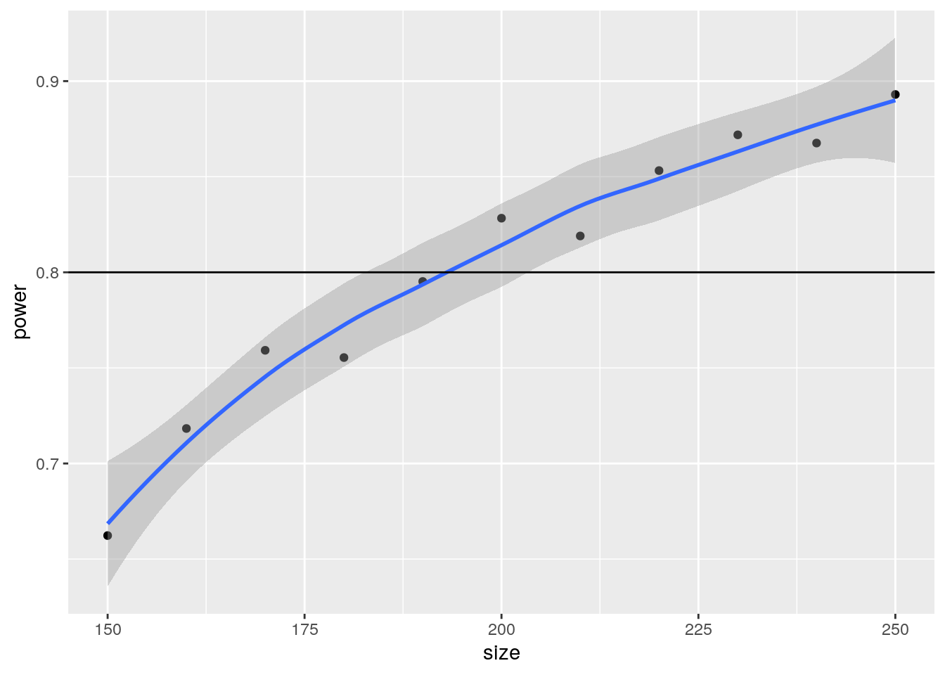
Alternatively, we can fit a linear regression model where we predict power as a function of sample size using linear and quadratic effects:
n = \theta_0 + \theta_1 (1 - \beta) + \theta_2 (1 - \beta)^2
# Fitting the model
power_model <- glm(
  size ~ power + I(power^2),
  data = simulations, family = gaussian()
)

# Printing the results
summary(power_model)
Call:
glm(formula = size ~ power + I(power^2), family = gaussian(),
    data = simulations)

Coefficients:
            Estimate Std. Error t value Pr(>|t|)
(Intercept)    632.5      232.9   2.715  0.02644 *
power        -1590.3      598.1  -2.659  0.02885 *
I(power^2)    1301.0      381.6   3.410  0.00923 **
---
Signif. codes:  0 '***' 0.001 '**' 0.01 '*' 0.05 '.' 0.1 ' ' 1

(Dispersion parameter for gaussian family taken to be 34.83159)

    Null deviance: 11000.00  on 10  degrees of freedom
Residual deviance:   278.65  on  8  degrees of freedom
AIC: 74.769

Number of Fisher Scoring iterations: 2
# Predict
predict(power_model, newdata = data.frame(power = .8), type = "response") |>
ceiling() 1
193 According to our simulation study, the closest to our 80% power is using a sample size equal to 193, which is very close to the analytical solution of 194.
As a final comment for this example, remember that the more simulations the better.