Exponential Random Graph Models [ERGMs] can represent a variety of network classes. We often look at “regular” social networks like students in schools, colleagues in the workplace, or families. Nonetheless, some social networks we study have features that restrict how connections can occur. Typical examples are bi-partite graphs and multilevel networks. There are two classes of vertices in bi-partite networks, and ties can only occur between classes. On the other hand, Multilevel networks may feature multiple classes with inter-class ties somewhat restricted. In both cases, structural constraints exist, meaning that some configurations may not be plausible.
Mathematically, what we are trying to do is, instead of assuming that all network configurations are possible:
\left\{\mathbf{y} \in \mathcal{Y}: y_{ij} = 0, \forall i = j\right\}
we want to go a bit further avoiding loops, namely:
where C is a constraint, for example, only networks with no triangles. The ergm R package has built-in capabilities to deal with some of these cases. Nonetheless, we can specify models with arbitrary structural constraints built into the model. The key is in using offset terms.
Example 1: Interlocking egos and disconnected alters
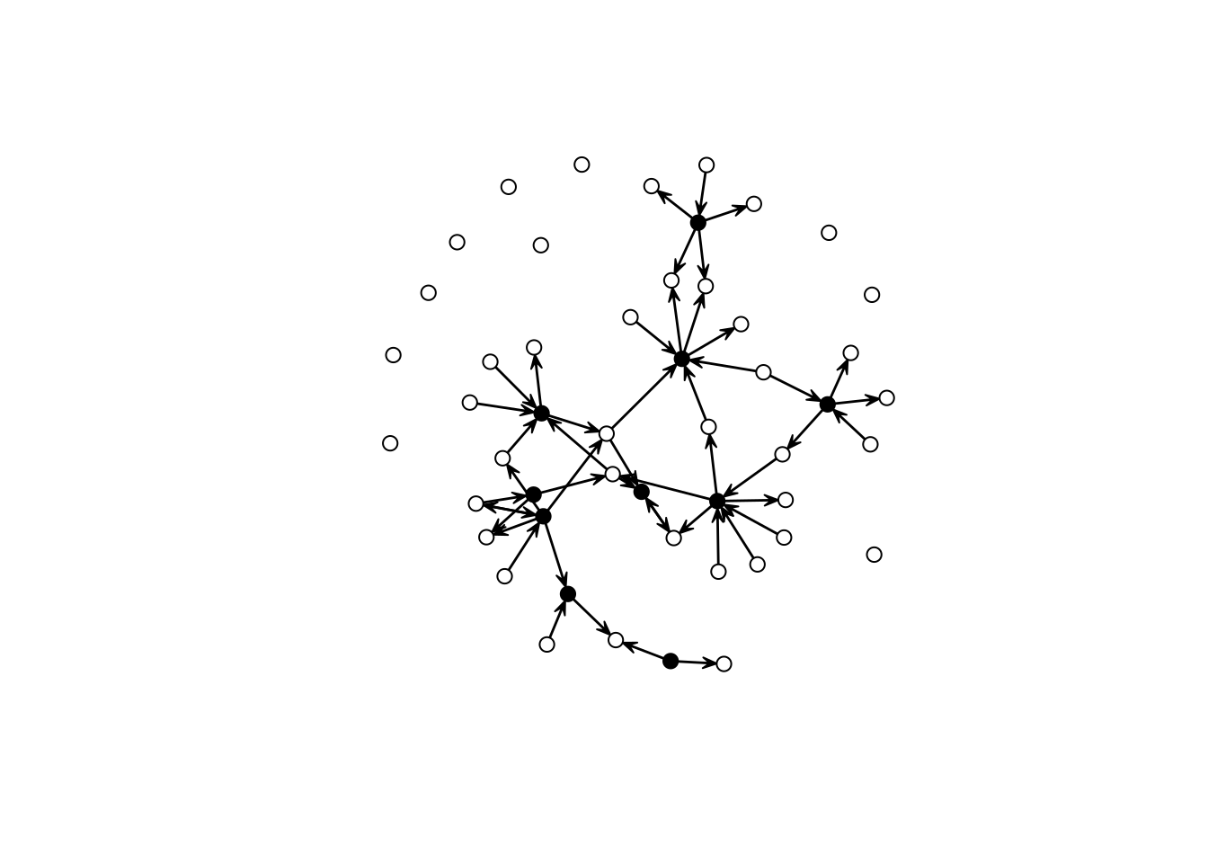
Imagine that we have two sets of vertices. The first, group E, are egos part of an egocentric study. The second group, called A, is composed of people mentioned by egos in E but were not surveyed. Assume that individuals in A can only connect to individuals in E; moreover, individuals in E have no restrictions on connecting. In other words, only two types of ties exist: E-E and A-E. The question is now, how can we enforce such a constraint in an ERGM?
Using offsets, and in particular, setting coefficients to -Inf provides an easy way to restrict the support set of ERGMs. For example, if we wanted to constrain the support to include networks with no triangles, we would add the term offset(triangle) and use the option offset.coef = -Inf to indicate that realizations including triangles are not possible. Using R:
In this model, a Bernoulli graph, we reduce the sample space to networks with no triangles. In our example, such a statistic should only take non-zero values whenever ties within the A class happen. We can use the nodematch() term to do that. Formally
This statistic will sum over all ties in which source (i) and target (j)’s X attribute is equal. One way to make this happen is by creating an auxiliary variable that equals, e.g., 0 for all vertices in A, and a unique value different from zero otherwise. For example, if we had 2 As and three Es, the data would look something like this: \{0,0,1,2,3\}. The following code block creates an empty graph with 50 nodes, 10 of which are in group E (ego).
library(ergm, quietly =TRUE)library(sna, quietly =TRUE)n <-50n_egos <-10net <-as.network(matrix(0, ncol = n, nrow = n), directed =TRUE)# Let's assing the groupsnet %v%"is.ego"<-c(rep(TRUE, n_egos), rep(FALSE, n - n_egos))net %v%"is.ego"
To create the auxiliary variable, we will use the following function:
# Function that creates an aux variable for the ergm modelmake_aux_var <-function(my_net, is_ego_dummy) { n_vertex <-length(my_net %v% is_ego_dummy) n_ego_ <-sum(my_net %v% is_ego_dummy)# Creating an auxiliary variable to identify the non-informant non-informant ties my_net %v%"aux_var"<-ifelse(!my_net %v% is_ego_dummy, 0, 1:(n_vertex - n_ego_) ) my_net}
Calling the function in our data results in the following:
net <-make_aux_var(net, "is.ego")# Taking a look over the first 15 rows of datacbind(Is_Ego = net %v%"is.ego",Aux = net %v%"aux_var") |>head(n =15)
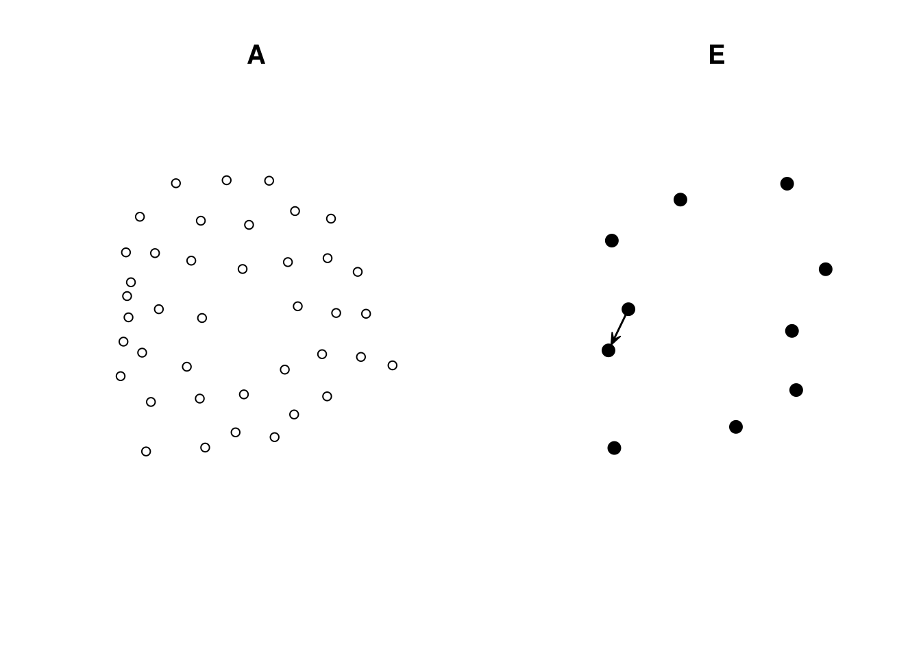
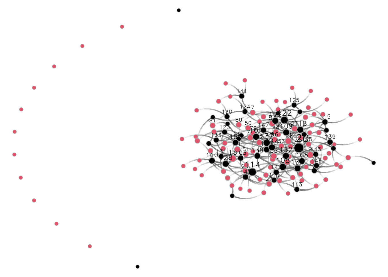
As you can see, this network has only ties of the type E-E and A-E. We can double-check by (i) looking at the counts and (ii) visualizing each induced-subgraph separately:
# Figuresop <-par(mfcol =c(1, 2))gplot(net_of_alters, vertex.col = net_of_alters %v%"is.ego", main ="A")gplot(net_of_egos, vertex.col = net_of_egos %v%"is.ego", main ="E")
par(op)
Now, to fit an ERGM with this constraint, we simply need to make use of the offset terms. Here is an example:
ans <-ergm( net_sim ~ edges +offset(nodematch("aux_var")), # The model (notice the offset)offset.coef =-Inf# The offset coefficient )## Starting maximum pseudolikelihood estimation (MPLE):## Obtaining the responsible dyads.## Evaluating the predictor and response matrix.## Maximizing the pseudolikelihood.## Finished MPLE.## Evaluating log-likelihood at the estimate.summary(ans)## Call:## ergm(formula = net_sim ~ edges + offset(nodematch("aux_var")), ## offset.coef = -Inf)## ## Maximum Likelihood Results:## ## Estimate Std. Error MCMC % z value Pr(>|z|) ## edges -3.0829 0.1638 0 -18.83 <1e-04 ***## offset(nodematch.aux_var) -Inf 0.0000 0 -Inf <1e-04 ***## ---## Signif. codes: 0 '***' 0.001 '**' 0.01 '*' 0.05 '.' 0.1 ' ' 1## ## Null Deviance: 3396.4 on 2450 degrees of freedom## Residual Deviance: 320.2 on 2448 degrees of freedom## ## AIC: 322.2 BIC: 327 (Smaller is better. MC Std. Err. = 0)## ## The following terms are fixed by offset and are not estimated:## `offset(nodematch.aux_var)` ##
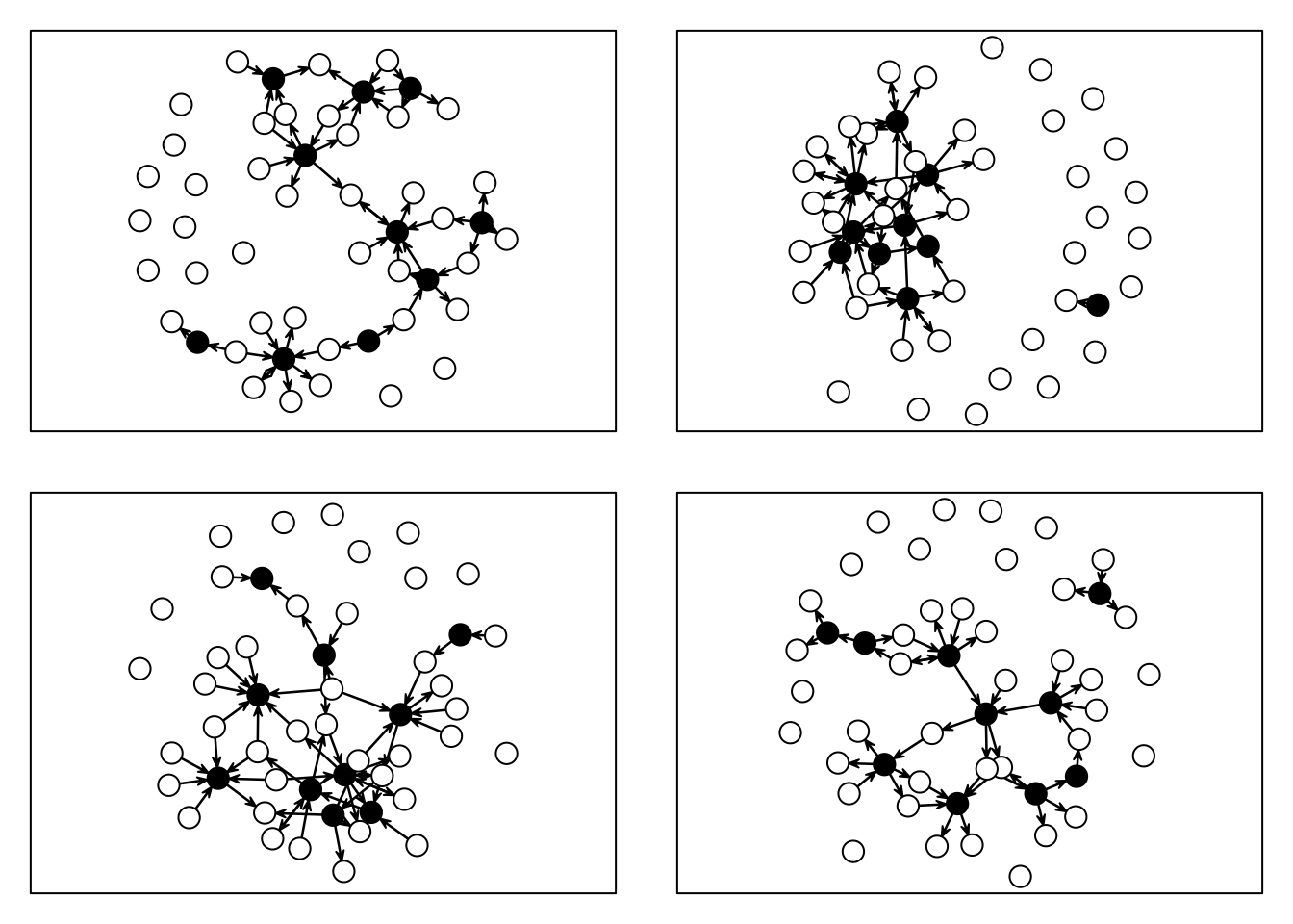
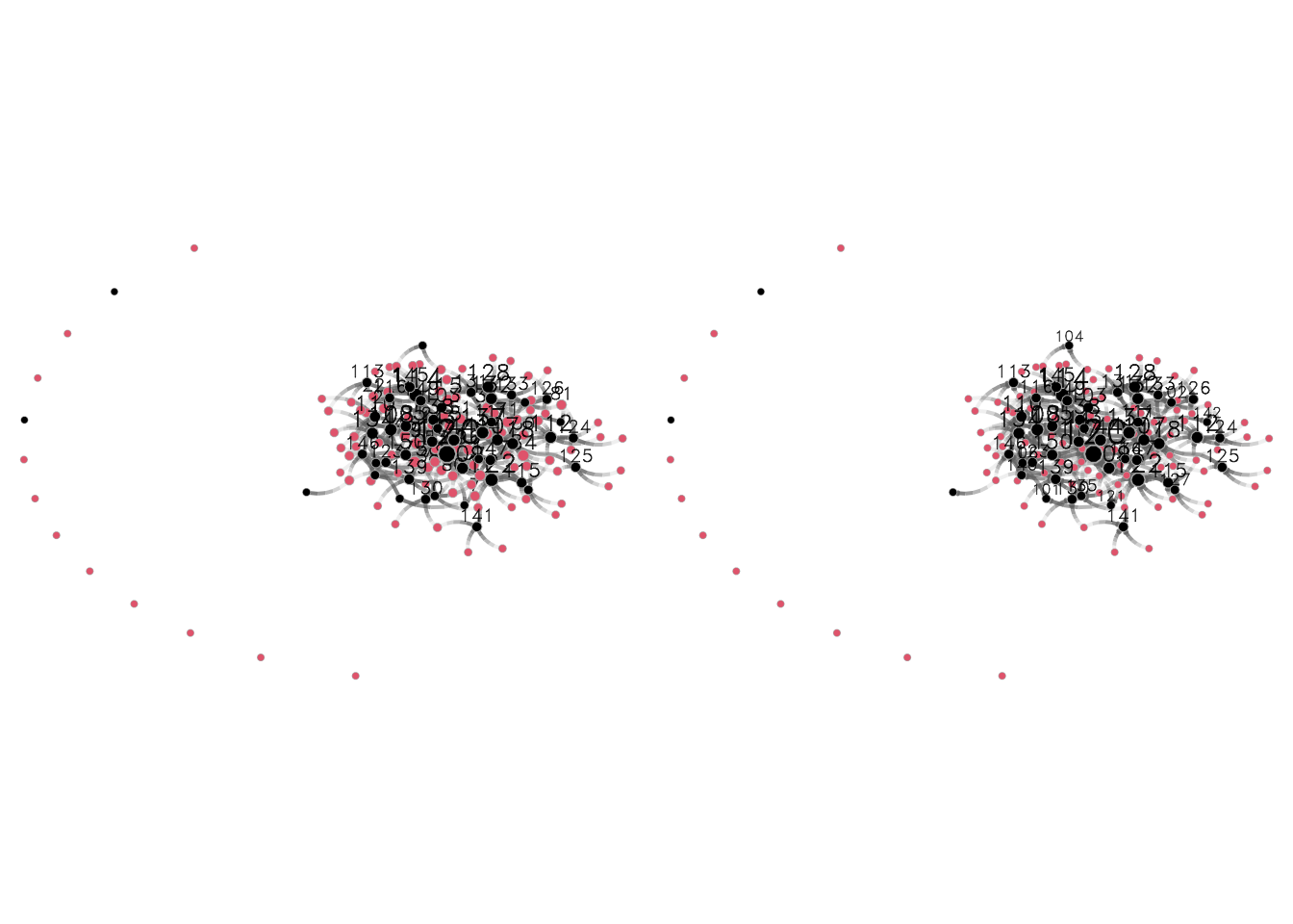
This ERGM model–which by the way only featured dyadic-independent terms, and thus can be reduced to a logistic regression–restricts the support by excluding all networks in which ties within the class A exists. To finalize, let’s look at a few simulations based on this model:
set.seed(1323)op <-par(mfcol =c(2,2), mar =rep(1, 4))for (i in1:4) {gplot(simulate(ans), vertex.col = net %v%"is.ego", vertex.cex =2)box()}
par(op)
All networks with no ties between A nodes.
Example 2: Bi-partite networks
In the case of bipartite networks (sometimes called affiliation networks,) we can use ergm’s terms for bipartite graphs to corroborate what we discussed here. For example, the two-star term. Let’s start simulating a bipartite network using the edges and two-star parameters. Since the k-star term is usually complex to fit (tends to generate degenerate models,) we will take advantage of the Log() transformation function in the ergm package to smooth the term.1
The bipartite network that we will be simulating will have 100 actors and 50 entities. Actors, which we will map to the first level of the ergm terms, this is, b1starb1nodematch, etc. will send ties to the entities, the second level of the bipartite ERGM. To create a bipartite network, we will create an empty matrix of size nactors x nentitites; thus, actors are represented by rows and entities by columns.
# Parameters for the simulationnactors <-100nentities <-floor(nactors/2)n <- nactors + nentities# Creating an empty bipartite network (baseline)net_b <-network(matrix(0, nrow = nactors, ncol = nentities), bipartite =TRUE)# Simulating the bipartite ERGM,net_b <-simulate(net_b ~ edges +Log(~b1star(2)), coef =c(-3, 1.5), seed =55)
Notice that the first nactors vertices in the network are the actors, and the remaining are the entities. Now, although the ergm package features bipartite network terms, we can still fit a bipartite ERGM without explicitly declaring the graph as such. In such case, the b1star(2) term of a bipartite network is equivalent to an ostar(2) in a directed graph. Likewise, b2star(2) in a bipartite graph matches the istar(2) term in a directed graph. This information will be relevant when fitting the ERGM. Let’s transform the bipartite network into a directed graph. The following code block does so:
# Identifying the edgesnet_not_b <-which(as.matrix(net_b) !=0, arr.ind =TRUE)# We need to offset the endpoint of the ties by nactors# so that the ids go from 1 through (nactors + nentitites)net_not_b[,2] <- net_not_b[,2] + nactors# The resulting graph is a directed networknet_not_b <-network(net_not_b, directed =TRUE)
Now we are almost done. As before, we need to use node-level covariates to put the constraints in our model. For this ERGM to reflect an ERGM on a bipartite network, we need two constraints:
Only ties from actors to entities are allowed, and
entities can only receive ties.
The corresponding offset terms for this model are: nodematch("is.actor") ~ -Inf, and nodeocov("isnot.actor") ~ -Inf. Mathematically:
In other words, we are setting that ties between nodes of the same class are forbidden, and outgoing ties are forbidden for entities. Let’s create the vertex attributes needed to use the aforementioned terms:
# Looking at the countssummary(net_b ~ edges +b1star(2) +b2star(2))
  edges b1star2 b2star2
    245     313     645
summary(net_not_b ~ edges +ostar(2) +istar(2))
 edges ostar2 istar2
   245    313    645
With the two networks matching, we can now fit the ERGMs with and without offset terms and compare the results between the two models:
# ERGM with a bipartite graphres_b <-ergm(# Main formula net_b ~ edges +Log(~b1star(2)),# Control parameterscontrol =control.ergm(seed =1) )
Warning: 'glpk' selected as the solver, but package 'Rglpk' is not available;
falling back to 'lpSolveAPI'. This should be fine unless the sample size and/or
the number of parameters is very big.
# ERGM with a digraph with constraintsres_not_b <-ergm(# Main formula net_not_b ~ edges +Log(~ostar(2)) +# Offset terms offset(nodematch("is.actor")) +offset(nodeocov("isnot.actor")),offset.coef =c(-Inf, -Inf),# Control parameterscontrol =control.ergm(seed =1) )
Here are the estimates (using the texreg R package for a prettier output):
As expected, both models yield the “same” estimate. The minor differences observed between the models are how the ergm package performs the sampling. In particular, in the bipartite case, ergm has special routines for making the sampling more efficient, having a higher acceptance rate than that of the model in which the bipartite graph was not explicitly declared. We can tell this by inspecting rejection rates:
The ERGM fitted with the offset terms has a much higher rejection rate than that of the ERGM fitted with the bipartite ERGM.
Finally, the fact that we can fit ERGMs using offset does not mean that we need to use it ALL the time. Unless there is a very good reason to go around ergm’s capabilities, I wouldn’t recommend fitting bipartite ERGMs as we just did, as the authors of the package have included (MANY) features to make our job easier.
After writing this example, it became apparent the use of the Log() transformation function may not be ideal. Since many terms used in ERGMs can be zero, e.g., triangles, the term Log(~ ostar(2)) is undefined when ostar(2) = 0. In practice, the ERGM package sets a lower limit for the log of 0, so, instead of having Log(0) ~ -Inf, they set it to be a really large negative number. This causes all sorts of issues to the estimates; in our example, an overestimation of the population parameter and a positive log-likelihood. Therefore, I wouldn’t recommend using this transformation too often.↩︎