library(ergm)
library(netplot)
data("sampson")
nplot(samplike)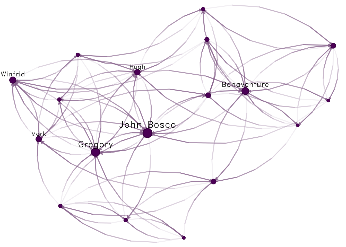
I strongly suggest reading the vignette in the ergm R package.
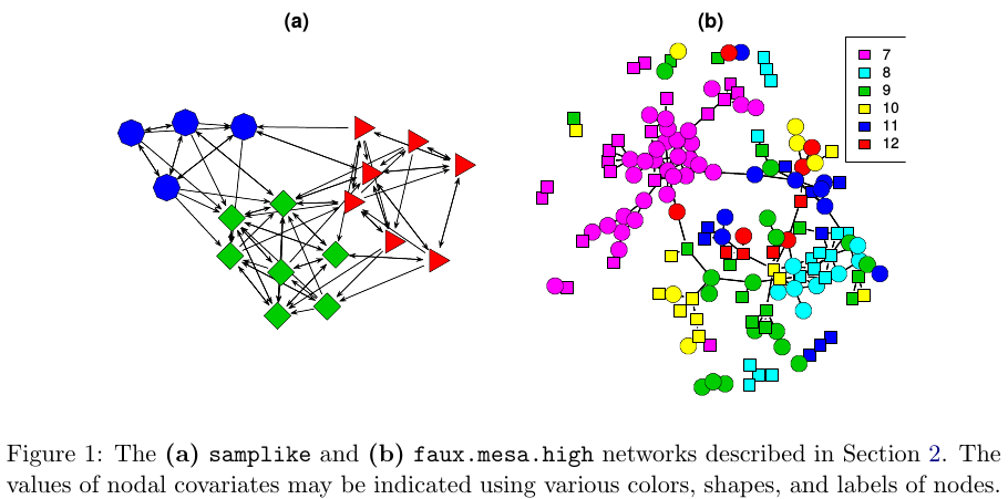
vignette("ergm", package="ergm")The purpose of ERGMs, in a nutshell, is to describe parsimoniously the local selection forces that shape the global structure of a network. To this end, a network dataset, like those depicted in Figure 1, may be considered as the response in a regression model, where the predictors are things like “propensity for individuals of the same sex to form partnerships” or “propensity for individuals to form triangles of partnerships”. In Figure 1(b), for example, it is evident that the individual nodes appear to cluster in groups of the same numerical labels (which turn out to be students’ grades, 7 through 12); thus, an ERGM can help us quantify the strength of this intra-group effect.
In a nutshell, we use ERGMs as a parametric interpretation of the distribution of \mathbf{Y}, which takes the canonical form:
{\mathbb{P}_{\mathcal{Y}}\left(\mathbf{Y}=\mathbf{y};\mathbf{\theta}\right) } = \frac{\text{exp}\left\{\theta^{\text{T}}\mathbf{g}(\mathbf{y})\right\}}{\kappa\left(\theta, \mathcal{Y}\right)},\quad\mathbf{y}\in\mathcal{Y} \tag{9.1}
Where \theta\in\Omega\subset\mathbb{R}^q is the vector of model coefficients and \mathbf{g}(\mathbf{y}) is a q-vector of statistics based on the adjacency matrix \mathbf{y}.
Model Equation 9.1 may be expanded by replacing \mathbf{g}(\mathbf{y}) with \mathbf{g}(\mathbf{y}, \mathbf{X}) to allow for additional covariate information \mathbf{X} about the network. The denominator \kappa\left(\theta,\mathcal{Y}\right) = \sum_{\mathbf{y}\in\mathcal{Y}}\text{exp}\left\{\theta^{\text{T}}\mathbf{g}(\mathbf{y})\right\} is the normalizing factor that ensures that equation Equation 9.1 is a legitimate probability distribution. Even after fixing \mathcal{Y} to be all the networks that have size n, the size of \mathcal{Y} makes this type of statistical model hard to estimate as there are N = 2^{n(n-1)} possible networks! (David R. Hunter et al. 2008)
Later developments include new dependency structures to consider more general neighborhood effects. These models relax the one-step Markovian dependence assumptions, allowing investigation of longer-range configurations, such as longer paths in the network or larger cycles (Pattison and Robins 2002). Models for bipartite (Faust and Skvoretz 1999) and tripartite (Mische and Robins 2000) network structures have been developed. (David R. Hunter et al. 2008, 9)
In the simplest case, ERGMs equate a logistic regression. By simple, I mean cases with no Markovian terms–motifs involving more than one edge–for example, the Bernoulli graph. In the Bernoulli graph, ties are independent, so the presence/absence of a tie between nodes i and j won’t affect the presence/absence of a tie between nodes k and l.
Let’s fit an ERGM using the sampson dataset in the ergm package.
library(ergm)
library(netplot)
data("sampson")
nplot(samplike)
Using ergm to fit a Bernoulli graph requires using the edges term, which counts how many ties are in the graph:
ergm_fit <- ergm(samplike ~ edges)
## Starting maximum pseudolikelihood estimation (MPLE):
## Obtaining the responsible dyads.
## Evaluating the predictor and response matrix.
## Maximizing the pseudolikelihood.
## Finished MPLE.
## Evaluating log-likelihood at the estimate.
Since this is equivalent to a logistic regression, we can use the glm function to fit the same model. First, we need to prepare the data so we can pass it to glm:
y <- sort(as.vector(as.matrix(samplike)))
y <- y[-c(1:18)] # We remove the diagonal from the model, which is all 0.
y
##   [1] 0 0 0 0 0 0 0 0 0 0 0 0 0 0 0 0 0 0 0 0 0 0 0 0 0 0 0 0 0 0 0 0 0 0 0 0 0
##  [38] 0 0 0 0 0 0 0 0 0 0 0 0 0 0 0 0 0 0 0 0 0 0 0 0 0 0 0 0 0 0 0 0 0 0 0 0 0
##  [75] 0 0 0 0 0 0 0 0 0 0 0 0 0 0 0 0 0 0 0 0 0 0 0 0 0 0 0 0 0 0 0 0 0 0 0 0 0
## [112] 0 0 0 0 0 0 0 0 0 0 0 0 0 0 0 0 0 0 0 0 0 0 0 0 0 0 0 0 0 0 0 0 0 0 0 0 0
## [149] 0 0 0 0 0 0 0 0 0 0 0 0 0 0 0 0 0 0 0 0 0 0 0 0 0 0 0 0 0 0 0 0 0 0 0 0 0
## [186] 0 0 0 0 0 0 0 0 0 0 0 0 0 0 0 0 0 0 0 0 0 0 0 0 0 0 0 0 0 0 0 0 0 1 1 1 1
## [223] 1 1 1 1 1 1 1 1 1 1 1 1 1 1 1 1 1 1 1 1 1 1 1 1 1 1 1 1 1 1 1 1 1 1 1 1 1
## [260] 1 1 1 1 1 1 1 1 1 1 1 1 1 1 1 1 1 1 1 1 1 1 1 1 1 1 1 1 1 1 1 1 1 1 1 1 1
## [297] 1 1 1 1 1 1 1 1 1 1
We can now fit the GLM model:
glm_fit <- glm(y~1, family=binomial("logit"))The coefficients of both ERGM and GLM should match:
glm_fit
##
## Call:  glm(formula = y ~ 1, family = binomial("logit"))
##
## Coefficients:
## (Intercept)
##     -0.9072
##
## Degrees of Freedom: 305 Total (i.e. Null);  305 Residual
## Null Deviance:       367.2
## Residual Deviance: 367.2     AIC: 369.2
ergm_fit
##
## Call:
## ergm(formula = samplike ~ edges)
##
## Maximum Likelihood Coefficients:
##   edges
## -0.9072
Furthermore, in the case of the Bernoulli graph, we can get the estimate using the Logit function:
pr <- mean(y)
# Logit function:
# Alternatively we could have used log(pr) - log(1-pr)
qlogis(pr)
## [1] -0.9071582
Again, the same result. The Bernoulli graph is not the only ERGM model that can be fitted using a Logistic regression. Moreover, if all the terms of the model are non-Markov terms, ergm automatically defaults to a Logistic regression.
The ultimate goal is to perform statistical inference on the proposed model. In a standard setting, we could use Maximum Likelihood Estimation (MLE), which consists of finding the model parameters \theta that, given the observed data, maximize the likelihood of the model. For the latter, we generally use Newton’s method. Newton’s method requires computing the model’s log-likelihood, which can be challenging in ERGMs.
For ERGMs, since part of the likelihood involves a normalizing constant that is a function of all possible networks, this is not as straightforward as in the regular setting. Because of this, most estimation methods rely on simulations.
In statnet, the default estimation method is based on a method proposed by (Geyer and Thompson 1992), Markov-Chain MLE, which uses Markov-Chain Monte Carlo for simulating networks and a modified version of the Newton-Raphson algorithm to estimate the parameters.
The idea of MC-MLE for this family of statistical models is to approximate the expectation of normalizing constant ratios using the law of large numbers. In particular, the following:
\begin{align*} \frac{\kappa\left(\theta,\mathcal{Y}\right)}{\kappa\left(\theta_0,\mathcal{Y}\right)} & = \frac{ \sum_{\mathbf{y}\in\mathcal{Y}}\text{exp}\left\{\theta^{\text{T}}\mathbf{g}(\mathbf{y})\right\}}{ \sum_{\mathbf{y}\in\mathcal{Y}}\text{exp}\left\{\theta_0^{\text{T}}\mathbf{g}(\mathbf{y})\right\} } \\ & = \sum_{\mathbf{y}\in\mathcal{Y}}\left( % \frac{1}{% \sum_{\mathbf{y}\in\mathcal{Y}\text{exp}\left\{\theta_0^{\text{T}}\mathbf{g}(\mathbf{y})\right\}}% } \times % \text{exp}\left\{\theta^{\text{T}}\mathbf{g}(\mathbf{y})\right\} % \right) \\ & = \sum_{\mathbf{y}\in\mathcal{Y}}\left( % \frac{\text{exp}\left\{\theta_0^{\text{T}}\mathbf{g}(\mathbf{y})\right\}}{% \sum_{\mathbf{y}\in\mathcal{Y}\text{exp}\left\{\theta_0^{\text{T}}\mathbf{g}(\mathbf{y})\right\}}% } \times % \text{exp}\left\{(\theta - \theta_0)^{\text{T}}\mathbf{g}(\mathbf{y})\right\} % \right) \\ & = \sum_{\mathbf{y}\in\mathcal{Y}}\left( % {\mathbb{P}_{\times }\left(Y = y|\mathcal{Y}, \theta_0\right) }% \text{exp}\left\{(\theta - \theta_0)^{\text{T}}\mathbf{g}(\mathbf{y})\right\} % \right) \\ & = \text{E}_{\theta_0}\left(\text{exp}\left\{(\theta - \theta_0)^{\text{T}}\mathbf{g}(\mathbf{y})\right\} \right) \end{align*}
In particular, the MC-MLE algorithm uses this fact to maximize the log-likelihood ratio. The objective function itself can be approximated by simulating m networks from the distribution with parameter \theta_0:
l(\theta) - l(\theta_0) \approx (\theta - \theta_0)^{\text{T}}\mathbf{g}(\mathbf{y}_{obs}) - \text{log}{\left[\frac{1}{m}\sum_{i = 1}^m\text{exp}\left\{(\theta-\theta_0)^{\text{T}}\right\}\mathbf{g}(\mathbf{Y}_i)\right]}
For more details, see (David R. Hunter et al. 2008). A sketch of the algorithm follows:
Initialize the algorithm with an initial guess of \theta, call it \theta^{(t)} (must be a rather OK guess)
While (no convergence) do:
Using \theta^{(t)}, simulate M networks by means of small changes in the \mathbf{Y}_{obs} (the observed network). This part is done by using an importance-sampling method which weights each proposed network by its likelihood conditional on \theta^{(t)}
With the networks simulated, we can do the Newton step to update the parameter \theta^{(t)} (this is the iteration part in the ergm package): \theta^{(t)}\to\theta^{(t+1)}.
If convergence has been reached (which usually means that \theta^{(t)} and \theta^{(t + 1)} are not very different), then stop; otherwise, go to step a.
Lusher, Koskinen, and Robins (2013);Admiraal and Handcock (2006);Snijders (2002);Wang et al. (2009) provides details on the algorithm used by PNet (the same as the one used in RSiena), and Lusher, Koskinen, and Robins (2013) provides a short discussion on the differences between ergm and PNet.
ergm packageFrom the previous section:1
library(igraph)

library(dplyr)

load("03.rda")
In this section, we will use the ergm package (from the statnet suit of packages Handcock et al. (2023),) and the intergraph (Bojanowski 2023) package. The latter provides functions to go back and forth between igraph and network objects from the igraph and network packages respectively2
library(ergm)
library(intergraph)
As a rather important side note, the order in which R packages are loaded matters. Why is this important to mention now? Well, it turns out that at least a couple of functions in the network package have the same name as some functions in the igraph package. When the ergm package is loaded, since it depends on network, it will load the network package first, which will mask some functions in igraph. This becomes evident once you load ergm after loading igraph:
The following objects are masked from ‘package:igraph’:

  add.edges, add.vertices, %c%, delete.edges, delete.vertices, get.edge.attribute, get.edges,
  get.vertex.attribute, is.bipartite, is.directed, list.edge.attributes, list.vertex.attributes, %s%,
  set.edge.attribute, set.vertex.attribute
What are the implications of this? If you call the function list.edge.attributes for an object of class igraph R will return an error as the first function that matches that name comes from the network package! To avoid this you can use the double colon notation:
igraph::list.edge.attributes(my_igraph_object)
network::list.edge.attributes(my_network_object)
Using the asNetwork function, we can coerce the igraph object into a network object so we can use it with the ergm function:
# Creating the new network
network_111 <- intergraph::asNetwork(ig_year1_111)

# Running a simple ergm (only fitting edge count)
ergm(network_111 ~ edges)
## Warning in ergm.getnetwork(formula): This network contains loops
## Starting maximum pseudolikelihood estimation (MPLE):
## Obtaining the responsible dyads.
## Evaluating the predictor and response matrix.
## Maximizing the pseudolikelihood.
## Finished MPLE.
## Evaluating log-likelihood at the estimate.
##
## Call:
## ergm(formula = network_111 ~ edges)
##
## Maximum Likelihood Coefficients:
##  edges
## -4.734
So what happened here? We got a warning. It turns out that our network has loops (didn’t think about it before!). Let’s take a look at that with the which_loop function
E(ig_year1_111)[which_loop(ig_year1_111)]
## + 1/2638 edge from 010b2e5 (vertex names):
## [1] 1110111->1110111
We can get rid of these using the igraph::-.igraph. Let’s remove the isolates using the same operator
# Creating the new network
network_111 <- ig_year1_111

# Removing loops
network_111 <- network_111 - E(network_111)[which(which_loop(network_111))]

# Removing isolates
network_111 <- network_111 - which(degree(network_111, mode = "all") == 0)

# Converting the network
network_111 <- intergraph::asNetwork(network_111)
asNetwork(simplify(ig_year1_111)) ig_year1_111 |> simplify() |> asNetwork()
A problem that we have with this data is the fact that some vertices have missing values in the variables hispanic, female1, and eversmk1. For now, we will proceed by imputing values based on the averages:
for (v in c("hispanic", "female1", "eversmk1")) {
  tmpv <- network_111 %v% v
  tmpv[is.na(tmpv)] <- mean(tmpv, na.rm = TRUE) > .5
  network_111 %v% v <- tmpv
}
Let’s take a look at the network
nplot(
  network_111,
  vertex.color = ~ hispanic
  )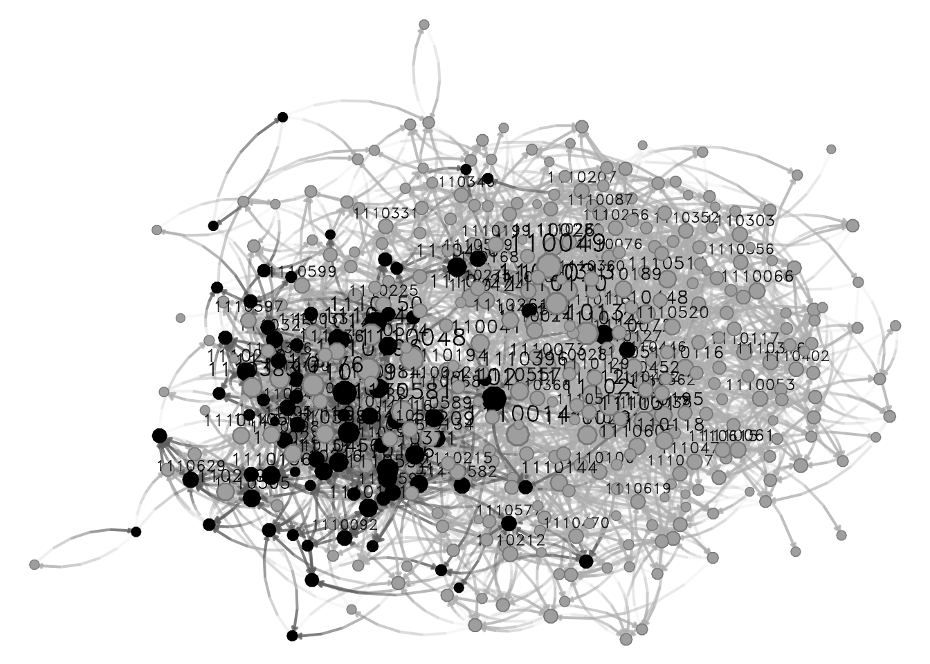
Coloring by hispanic, we can see that nodes seem to be clustered by this attribute. Visual inspection in network science can be very useful, but, in order to make more formal statements, we need to use statistical models; this is where ERGMs shine.
Although there is no silver bullet for estimating these models, the following workflow has worked for me in the past:
Estimate the simplest model, adding one variable at a time.
After each estimation, run the mcmc.diagnostics function to see how good (or bad) behaved the chains are.
Run the gof function and verify how good the model matches the network’s structural statistics.
What to use:
control.ergms: Maximum number of iterations, seed for Pseudo-RNG, how many cores
ergm.constraints: Where to sample the network from. Gives stability and (in some cases) faster convergence as by constraining the model you are reducing the sample size.
Here is an example of a couple of models that we could compare
Notice that this document may not include the usual messages that the ergm command generates during the estimation procedure. This is just to make it more printable-friendly.
ans0 <- ergm(
  network_111 ~
    edges +
    nodematch("hispanic") +
    nodematch("female1") +
    nodematch("eversmk1") +
    mutual,
  control = control.ergm(
    seed        = 1,
    MCMLE.maxit = 10,
    parallel    = 4,
    CD.maxit    = 10
    )
  )
## Warning: 'glpk' selected as the solver, but package 'Rglpk' is not available;
## falling back to 'lpSolveAPI'. This should be fine unless the sample size and/or
## the number of parameters is very big.In a previous version of the book we used the bd constraint to limit the maximum number of outgoing ties to 19. Although this is a reasonable constraint (as the sample may have been restricted by construction), the current version of the ERGM package returns a warning and shows the GOF statistics with switched signs (negative AIC and BIC, and positive Loglikelihood).
So what are we doing here:
The model is controlling for:
edges Number of edges in the network (as opposed to its density)
nodematch("some-variable-name-here") Includes a term that controls for homophily/heterophily
mutual Number of mutual connections between (i, j), (j, i). This can be related to, for example, triadic closure.
For more on control parameters, see Morris, Handcock, and Hunter (2008). The next model consists of a simpler version. Excluding the mutual term leads to an ERGM with no Markov terms, meaning that all the sufficient statistics are functions of individual edges rather than configurations involving multiple edges. The mutual term, by contrast, involves pairs of ties (i \to j and j \to i), which is an example of a Markov term. Models with only non-Markov terms reduce to a logistic regression, which is why the fitting process avoids using MCMC:
ans1 <- ergm(
  network_111 ~
    edges +
    nodematch("hispanic") +
    nodematch("female1") +
    nodematch("eversmk1")
    ,
  control = control.ergm(
    seed        = 1,
    MCMLE.maxit = 10,
    parallel    = 4,
    CD.maxit    = 10
    )
  )
Finally, we can try incorporating a more complex term, for example, the geometrically weighted edge-wise shared partners (gwesp) term. This term is akin to triadic closure, but it is easier to estimate. Moreover, to ease the estimation process, it is recommended to add the geometrically weighted dyad-wise shared partners (gwdsp) term too. Both terms include a decay parameter; for simplicity, both will be fixed and set to be 0.5 (values between 0.25 and 1.5 are common). For more on this, see David R. Hunter (2007).
ans2 <- ergm(
  network_111 ~
    edges +
    nodematch("hispanic") +
    nodematch("female1") +
    nodematch("eversmk1") +
    mutual +
    gwesp(decay = 0.5, fixed = TRUE) +
    gwdsp(decay = 0.5, fixed = TRUE)
    ,
  control = control.ergm(
    seed        = 1,
    MCMLE.maxit = 10,
    parallel    = 4,
    CD.maxit    = 10
    )
  )
Now, a nice trick to see all regressions in the same table, we can use the texreg package (Leifeld 2013) which supports ergm ouputs!
library(texreg)
## Version:  1.39.5
## Date:     2025-12-21
## Author:   Philip Leifeld (University of Manchester)
##
## Consider submitting praise using the praise or praise_interactive functions.
## Please cite the JSS article in your publications -- see citation("texreg").
screenreg(list(ans0, ans1, ans2))
##
## ================================================================
##                      Model 1        Model 2        Model 3
## ----------------------------------------------------------------
## edges                    -5.62 ***      -5.49 ***      -4.73 ***
##                          (0.05)         (0.06)         (0.07)
## nodematch.hispanic        0.22 ***       0.30 ***       0.16 ***
##                          (0.04)         (0.05)         (0.03)
## nodematch.female1         0.87 ***       1.16 ***       0.47 ***
##                          (0.04)         (0.05)         (0.03)
## nodematch.eversmk1        0.33 ***       0.45 ***       0.23 ***
##                          (0.04)         (0.04)         (0.03)
## mutual                    4.10 ***                      2.72 ***
##                          (0.07)                        (0.08)
## gwesp.OTP.fixed.0.5                                     1.34 ***
##                                                        (0.03)
## gwdsp.OTP.fixed.0.5                                    -0.11 ***
##                                                        (0.01)
## ----------------------------------------------------------------
## AIC                   22649.55       25135.63       20155.83
## BIC                   22699.89       25175.91       20226.31
## Log Likelihood       -11319.77      -12563.82      -10070.91
## ================================================================
## *** p < 0.001; ** p < 0.01; * p < 0.05
Or, if you are using rmarkdown, you can export the results using LaTeX or html, let’s try the latter to see how it looks like here:
library(texreg)
htmlreg(list(ans0, ans1, ans2))| Model 1 | Model 2 | Model 3 | |
|---|---|---|---|
| edges | -5.62*** | -5.49*** | -4.73*** |
| (0.05) | (0.06) | (0.07) | |
| nodematch.hispanic | 0.22*** | 0.30*** | 0.16*** |
| (0.04) | (0.05) | (0.03) | |
| nodematch.female1 | 0.87*** | 1.16*** | 0.47*** |
| (0.04) | (0.05) | (0.03) | |
| nodematch.eversmk1 | 0.33*** | 0.45*** | 0.23*** |
| (0.04) | (0.04) | (0.03) | |
| mutual | 4.10*** | 2.72*** | |
| (0.07) | (0.08) | ||
| gwesp.OTP.fixed.0.5 | 1.34*** | ||
| (0.03) | |||
| gwdsp.OTP.fixed.0.5 | -0.11*** | ||
| (0.01) | |||
| AIC | 22649.55 | 25135.63 | 20155.83 |
| BIC | 22699.89 | 25175.91 | 20226.31 |
| Log Likelihood | -11319.77 | -12563.82 | -10070.91 |
| ***p < 0.001; **p < 0.01; *p < 0.05 | |||
Before we go to the next section, let’s make some comments on what we see in the table:
Of the three models, the last one is the best in terms of smallest AIC and BIC, and largest Loglikelihood.
All the nodematch terms are significant and positive, which means that we have homophily by hispanic, female1, and eversmk1.
The mutual term is significant, positive, and large (~4). This indicates a strong tendency for individuals to befriend each other.
The gwesp term is positive and significant. The interpretation of this term is not always simple. Generally, we say that a positive gwesp term means that there is a tendency for triadic closure.
In raw terms, once each chain has reached stationary distribution, we can say that there are no problems with autocorrelation and that each sample point is iid. The latter implies that, since we are running the model with more than one chain, we can use all the samples (chains) as a single dataset.
Recent changes in the ergm estimation algorithm mean that these plots can no longer be used to ensure that the mean statistics from the model match the observed network statistics. For that functionality, please use the GOF command:
gof(object, GOF=~model).—?ergm::mcmc.diagnostics
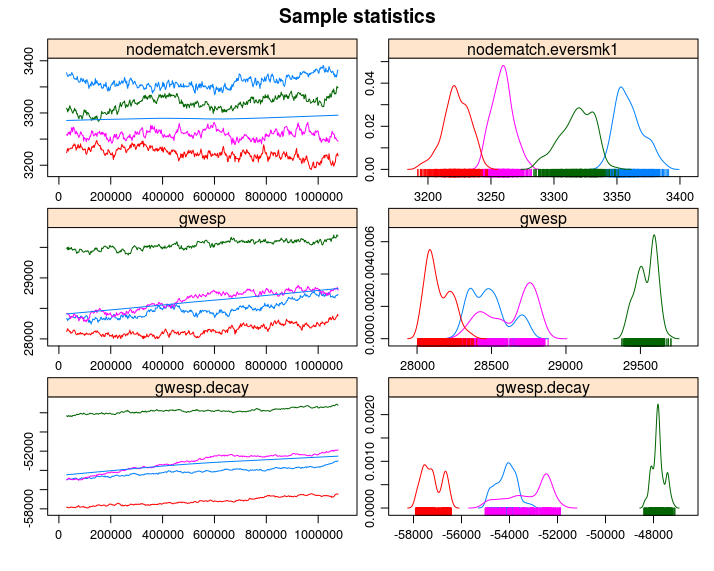
Since ans2 is the best model, let’s look at the GOF statistics. First, let’s see how the MCMC did. We can use the mcmc.diagnostics function included in the package. The function is a wrapper of a couple of functions from the coda package (Plummer et al. 2006), which are called upon the $sample object holding the centered statistics from the sampled networks. At first, it can be confusing to look at the $sample object; it neither matches the observed statistics nor the coefficients.
When calling mcmc.diagnostics(ans2, centered = FALSE), you will see many outputs, including a couple of plots showing the trace and posterior distribution of the uncentered statistics (centered = FALSE). The following code chunks will reproduce the output from the mcmc.diagnostics function step by step using the coda package. First, we need to uncenter the sample object:
# Getting the centered sample
sample_centered <- ans2$sample

# Getting the observed statistics and turning it into a matrix so we can add it
# to the samples
observed <- summary(ans2$formula)
observed <- matrix(
  observed,
  nrow  = nrow(sample_centered[[1]]),
  ncol  = length(observed),
  byrow = TRUE
  )

# Now we uncenter the sample
sample_uncentered <- lapply(sample_centered, function(x) {
  x + observed
})

# We have to make it an mcmc.list object
sample_uncentered <- coda::mcmc.list(sample_uncentered)
Under the hood:
summary(sample_uncentered)
##
## Iterations = 327680:5963776
## Thinning interval = 32768
## Number of chains = 4
## Sample size per chain = 173
##
## 1. Empirical mean and standard deviation for each variable,
##    plus standard error of the mean:
##
##                        Mean     SD Naive SE Time-series SE
## edges                2471.9  63.94    2.430          6.221
## nodematch.hispanic   1829.8  59.02    2.244          7.099
## nodematch.female1    1874.4  71.09    2.703          8.346
## nodematch.eversmk1   1755.6  58.02    2.206          6.746
## mutual                481.9  27.72    1.054          3.379
## gwesp.OTP.fixed.0.5  1762.6 113.98    4.333         13.574
## gwdsp.OTP.fixed.0.5 13175.1 644.91   24.516         66.387
##
## 2. Quantiles for each variable:
##
##                        2.5%   25%   50%   75% 97.5%
## edges                2347.3  2431  2469  2510  2605
## nodematch.hispanic   1718.3  1791  1827  1867  1955
## nodematch.female1    1736.0  1827  1871  1928  2016
## nodematch.eversmk1   1654.3  1714  1752  1794  1879
## mutual                429.3   462   481   500   542
## gwesp.OTP.fixed.0.5  1540.9  1684  1760  1835  2013
## gwdsp.OTP.fixed.0.5 11958.3 12737 13137 13596 14488coda::crosscorr(sample_uncentered)
## edges nodematch.hispanic nodematch.female1
## edges 1.0000000 0.8566830 0.8770210
## nodematch.hispanic 0.8566830 1.0000000 0.7573169
## nodematch.female1 0.8770210 0.7573169 1.0000000
## nodematch.eversmk1 0.8229030 0.6949758 0.7455362
## mutual 0.7921269 0.7019044 0.7765035
## gwesp.OTP.fixed.0.5 0.8782943 0.7780147 0.8679069
## gwdsp.OTP.fixed.0.5 0.9678268 0.8370254 0.8591945
## nodematch.eversmk1 mutual gwesp.OTP.fixed.0.5
## edges 0.8229030 0.7921269 0.8782943
## nodematch.hispanic 0.6949758 0.7019044 0.7780147
## nodematch.female1 0.7455362 0.7765035 0.8679069
## nodematch.eversmk1 1.0000000 0.7067807 0.7820246
## mutual 0.7067807 1.0000000 0.8954091
## gwesp.OTP.fixed.0.5 0.7820246 0.8954091 1.0000000
## gwdsp.OTP.fixed.0.5 0.8098323 0.7688635 0.8575789
## gwdsp.OTP.fixed.0.5
## edges 0.9678268
## nodematch.hispanic 0.8370254
## nodematch.female1 0.8591945
## nodematch.eversmk1 0.8098323
## mutual 0.7688635
## gwesp.OTP.fixed.0.5 0.8575789
## gwdsp.OTP.fixed.0.5 1.0000000coda::autocorr(sample_uncentered)[[1]]
## , , edges
##
## edges nodematch.hispanic nodematch.female1 nodematch.eversmk1
## Lag 0 1.000000000 0.85174677 0.90035143 0.84731435
## Lag 32768 0.604509897 0.52958876 0.66467595 0.54146395
## Lag 163840 0.369212891 0.35412936 0.40011462 0.39283115
## Lag 327680 0.184463035 0.14706318 0.24305479 0.29114538
## Lag 1638400 0.009007472 -0.02631294 0.03456016 -0.04578478
## mutual gwesp.OTP.fixed.0.5 gwdsp.OTP.fixed.0.5
## Lag 0 0.83296982 0.9136663 0.97089215
## Lag 32768 0.68928494 0.6870541 0.57938173
## Lag 163840 0.45203629 0.4511364 0.36536136
## Lag 327680 0.12747154 0.1829741 0.15036241
## Lag 1638400 0.05607638 0.0292786 -0.01022981
##
## , , nodematch.hispanic
##
## edges nodematch.hispanic nodematch.female1 nodematch.eversmk1
## Lag 0 0.851746774 1.00000000 0.796948280 0.77244980
## Lag 32768 0.540210932 0.64168452 0.620791472 0.51899205
## Lag 163840 0.348421398 0.40142712 0.409478507 0.40705581
## Lag 327680 0.156894106 0.10147048 0.226595532 0.24435622
## Lag 1638400 0.007637041 -0.04655592 -0.007443898 -0.07226516
## mutual gwesp.OTP.fixed.0.5 gwdsp.OTP.fixed.0.5
## Lag 0 0.69025542 0.795564260 0.82655175
## Lag 32768 0.58418987 0.623959752 0.52242442
## Lag 163840 0.42435250 0.432709863 0.35047668
## Lag 327680 0.11948613 0.174673754 0.13223947
## Lag 1638400 0.05123385 0.007771714 -0.02509792
##
## , , nodematch.female1
##
## edges nodematch.hispanic nodematch.female1 nodematch.eversmk1
## Lag 0 0.90035143 0.796948280 1.00000000 0.79308088
## Lag 32768 0.60258009 0.536790742 0.73348572 0.56527326
## Lag 163840 0.32695326 0.324827911 0.37903351 0.38465484
## Lag 327680 0.11123941 0.111356563 0.21164986 0.27852000
## Lag 1638400 0.07516871 -0.002982911 0.09513563 -0.06106261
## mutual gwesp.OTP.fixed.0.5 gwdsp.OTP.fixed.0.5
## Lag 0 0.79999770 0.88951827 0.87107087
## Lag 32768 0.66026068 0.69041074 0.56750224
## Lag 163840 0.38096094 0.39655308 0.32909183
## Lag 327680 0.07195343 0.12801382 0.08708550
## Lag 1638400 0.11308394 0.09505784 0.04044172
##
## , , nodematch.eversmk1
##
## edges nodematch.hispanic nodematch.female1 nodematch.eversmk1
## Lag 0 0.84731435 0.7724498 0.79308088 1.0000000
## Lag 32768 0.54365021 0.5122084 0.63731624 0.6624233
## Lag 163840 0.31661036 0.3735145 0.38613833 0.4631210
## Lag 327680 0.12487907 0.1838576 0.21306300 0.2895293
## Lag 1638400 -0.04843904 -0.0871528 -0.05860075 -0.1732522
## mutual gwesp.OTP.fixed.0.5 gwdsp.OTP.fixed.0.5
## Lag 0 0.73949417 0.82596806 0.82962588
## Lag 32768 0.59917271 0.64206417 0.53636921
## Lag 163840 0.36156912 0.38961111 0.32502461
## Lag 327680 0.06513275 0.10756201 0.12157020
## Lag 1638400 -0.02126220 -0.05784788 -0.05300152
##
## , , mutual
##
## edges nodematch.hispanic nodematch.female1 nodematch.eversmk1
## Lag 0 0.832969818 0.6902554 0.79999770 0.73949417
## Lag 32768 0.655957685 0.5420351 0.68082349 0.60650896
## Lag 163840 0.453711697 0.3807566 0.46832909 0.47654529
## Lag 327680 0.189592365 0.1950812 0.25444882 0.34592646
## Lag 1638400 0.004326463 -0.0397559 0.03453263 -0.04956656
## mutual gwesp.OTP.fixed.0.5 gwdsp.OTP.fixed.0.5
## Lag 0 1.00000000 0.91166903 0.790126039
## Lag 32768 0.77089766 0.75016262 0.613992396
## Lag 163840 0.51073753 0.53492576 0.445401161
## Lag 327680 0.19116258 0.22568907 0.144338541
## Lag 1638400 0.01557354 0.02072621 -0.002615637
##
## , , gwesp.OTP.fixed.0.5
##
## edges nodematch.hispanic nodematch.female1 nodematch.eversmk1
## Lag 0 0.91366631 0.79556426 0.88951827 0.82596806
## Lag 32768 0.65221015 0.57748172 0.71103822 0.63534710
## Lag 163840 0.40355191 0.36375124 0.42906065 0.45848417
## Lag 327680 0.16182896 0.15751100 0.23871746 0.30543634
## Lag 1638400 0.02774368 -0.01550744 0.04360474 -0.05912761
## mutual gwesp.OTP.fixed.0.5 gwdsp.OTP.fixed.0.5
## Lag 0 0.91166903 1.00000000 0.88286005
## Lag 32768 0.75714027 0.74743488 0.62020864
## Lag 163840 0.47254922 0.48618158 0.40054594
## Lag 327680 0.14530942 0.18887509 0.12356707
## Lag 1638400 0.05355936 0.04005611 0.01544559
##
## , , gwdsp.OTP.fixed.0.5
##
## edges nodematch.hispanic nodematch.female1 nodematch.eversmk1
## Lag 0 0.97089215 0.82655175 0.87107087 0.82962588
## Lag 32768 0.56904543 0.49933571 0.63747170 0.51566990
## Lag 163840 0.31817376 0.32249022 0.37414872 0.32999678
## Lag 327680 0.15987338 0.11941690 0.21123819 0.24152798
## Lag 1638400 0.01040193 -0.02676337 0.01558998 -0.05445063
## mutual gwesp.OTP.fixed.0.5 gwdsp.OTP.fixed.0.5
## Lag 0 0.79012604 0.8828601 1.00000000
## Lag 32768 0.64720629 0.6437981 0.56197239
## Lag 163840 0.40245842 0.4041699 0.32130564
## Lag 327680 0.09213271 0.1437246 0.12697167
## Lag 1638400 0.06161009 0.0289774 -0.01011366“If the samples are drawn from the stationary distribution of the chain, the two means are equal and Geweke’s statistic has an asymptotically standard normal distribution. […] The Z-score is calculated under the assumption that the two parts of the chain are asymptotically independent, which requires that the sum of frac1 and frac2 be strictly less than 1.””
—?coda::geweke.diag
Let’s take a look at a single chain:
coda::geweke.diag(sample_uncentered)[[1]]
##
## Fraction in 1st window = 0.1
## Fraction in 2nd window = 0.5
##
##               edges  nodematch.hispanic   nodematch.female1  nodematch.eversmk1
##             -1.0828             -0.9888             -1.7401             -0.8217
##              mutual gwesp.OTP.fixed.0.5 gwdsp.OTP.fixed.0.5
## -1.4265 -1.1219 -0.8655Gelman and Rubin (1992) propose a general approach to monitoring convergence of MCMC output in which m > 1 parallel chains are run with starting values that are overdispersed relative to the posterior distribution. Convergence is diagnosed when the chains have ‘forgotten’ their initial values, and the output from all chains is indistinguishable. The gelman.diag diagnostic is applied to a single variable from the chain. It is based a comparison of within-chain and between-chain variances, and is similar to a classical analysis of variance. —?coda::gelman.diag
As a difference from the previous diagnostic statistic, this uses all chains simultaneously:
coda::gelman.diag(sample_uncentered)
## Potential scale reduction factors:
##
##                     Point est. Upper C.I.
## edges                     1.05       1.14
## nodematch.hispanic        1.02       1.04
## nodematch.female1         1.07       1.20
## nodematch.eversmk1        1.07       1.22
## mutual                    1.07       1.20
## gwesp.OTP.fixed.0.5       1.09       1.26
## gwdsp.OTP.fixed.0.5       1.06       1.18
##
## Multivariate psrf
##
## 1.15
As a rule of thumb, values in the [.9,1.1] are good.
One nice feature of the mcmc.diagnostics function is the nice trace and posterior distribution plots that it generates. If you have the R package latticeExtra (Sarkar and Andrews 2022), the function will override the default plots used by coda::plot.mcmc and use lattice instead, creating nicer-looking plots. The next code chunk calls the mcmc.diagnostic function, but we suppress the rest of the output (see figure ?fig-coda-plots).
# [2022-03-13] This line is failing for what it could be an ergm bug
# mcmc.diagnostics(ans0, center = FALSE) # Suppressing all the output
If we call the function mcmc.diagnostics, this message appears at the end:
MCMC diagnostics shown here are from the last round of simulation, prior to computation of final parameter estimates. Because the final estimates are refinements of those used for this simulation run, these diagnostics may understate model performance. To directly assess the performance of the final model on in-model statistics, please use the GOF command: gof(ergmFitObject, GOF=~model).
—
mcmc.diagnostics(ans0)
Not that bad (although the mutual term could do better)!3 First, observe that in the figure, we see four different lines; why is that? Since we were running in parallel using four cores, the algorithm ran four chains of the MCMC algorithm. An eyeball test is to see if all the chains moved at about the same place; in such a case, we can start thinking about model convergence from the MCMC perspective.
Once we are sure to have reach convergence on the MCMC algorithm, we can start thinking about how well does our model predicts the observed network’s proterties. Besides the statistics that define our ERGM, the gof function’s default behavior show GOF for:
Let’s take a look at it
# Computing and printing GOF estatistics
ans_gof <- gof(ans2)
ans_gof
##
## Goodness-of-fit for model statistics
##
## obs min mean max MC p-value
## edges 2475.000 2294.000 2423.050 2622.000 0.44
## nodematch.hispanic 1832.000 1675.000 1804.840 1944.000 0.66
## nodematch.female1 1879.000 1702.000 1810.930 1933.000 0.26
## nodematch.eversmk1 1755.000 1646.000 1731.830 1847.000 0.70
## mutual 486.000 410.000 465.890 527.000 0.64
## gwesp.OTP.fixed.0.5 1775.406 1530.405 1690.474 1905.719 0.48
## gwdsp.OTP.fixed.0.5 13187.633 11220.527 12642.571 14646.853 0.44
##
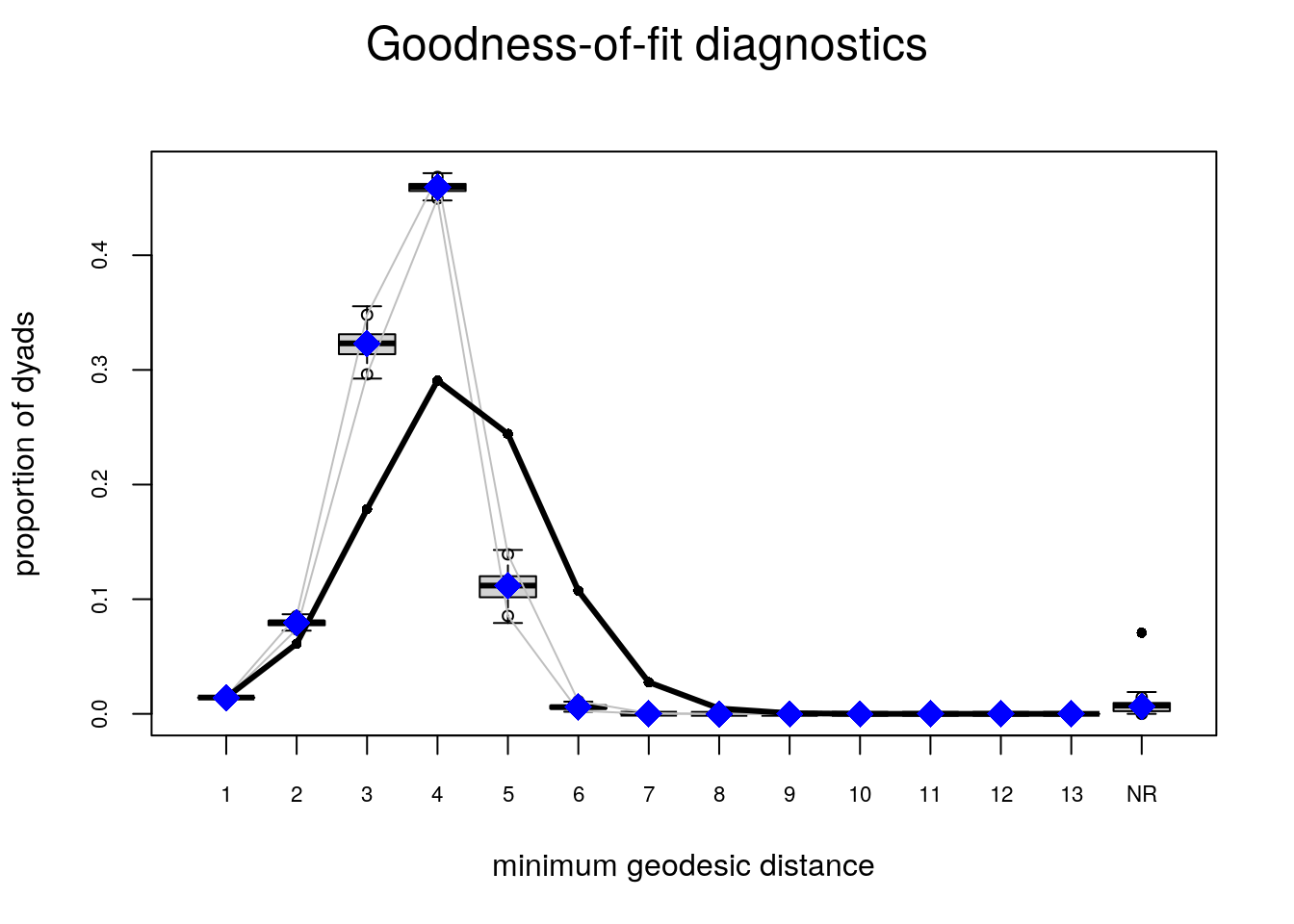
## Goodness-of-fit for minimum geodesic distance
##
## obs min mean max MC p-value
## 1 2475 2294 2423.05 2622 0.44
## 2 10672 9223 10480.93 12074 0.74
## 3 31134 30852 36074.17 41709 0.02
## 4 50673 61190 65958.18 71501 0.00
## 5 42563 35578 41259.49 48248 0.70
## 6 18719 5072 9728.74 14627 0.00
## 7 4808 444 1402.11 2760 0.00
## 8 822 16 174.57 888 0.02
## 9 100 0 21.66 353 0.08
## 10 7 0 2.40 54 0.16
## 11 0 0 0.25 8 1.00
## 12 0 0 0.01 1 1.00
## Inf 12333 2079 6780.44 11879 0.00
##
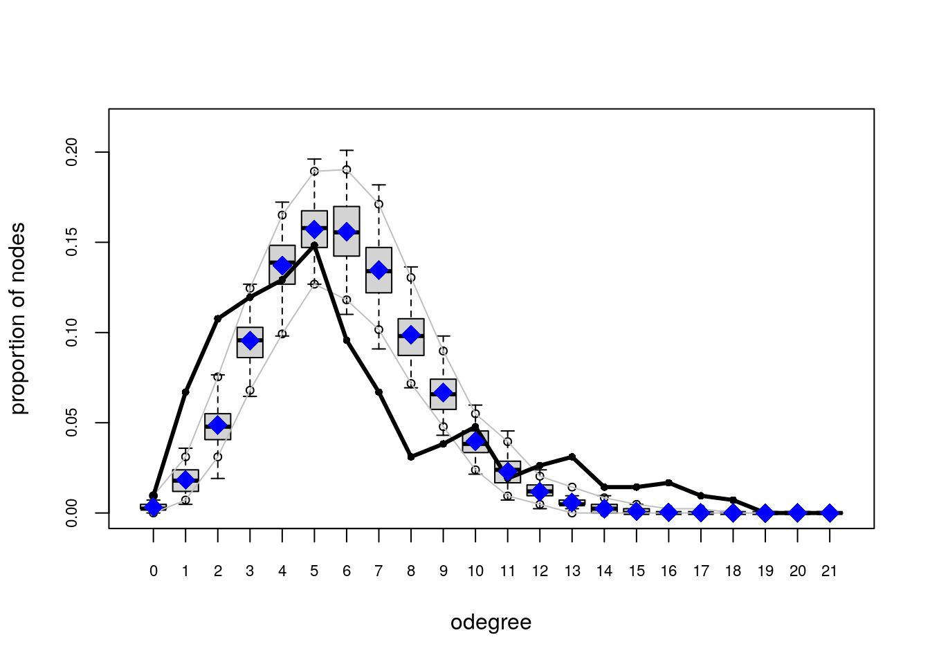
## Goodness-of-fit for out-degree
##
## obs min mean max MC p-value
## 0 4 3 7.65 14 0.28
## 1 28 11 19.93 30 0.14
## 2 45 20 33.48 51 0.08
## 3 50 27 43.75 59 0.42
## 4 54 30 51.34 65 0.64
## 5 62 35 52.02 71 0.24
## 6 40 36 50.11 71 0.16
## 7 28 33 44.18 58 0.00
## 8 13 23 35.64 50 0.00
## 9 16 16 27.49 38 0.04
## 10 20 9 19.90 34 1.00
## 11 8 5 13.51 21 0.10
## 12 11 3 8.70 17 0.44
## 13 13 0 4.49 14 0.02
## 14 6 0 3.00 7 0.12
## 15 6 0 1.42 5 0.00
## 16 7 0 0.79 3 0.00
## 17 4 0 0.30 2 0.00
## 18 3 0 0.18 2 0.00
## 19 0 0 0.06 1 1.00
## 20 0 0 0.06 1 1.00
##
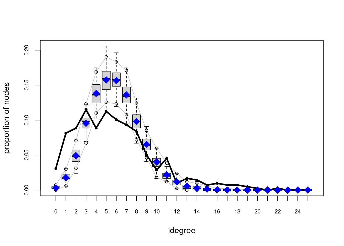
## Goodness-of-fit for in-degree
##
## obs min mean max MC p-value
## 0 13 2 7.48 13 0.08
## 1 34 10 19.25 30 0.00
## 2 37 26 34.83 46 0.82
## 3 48 31 44.19 61 0.54
## 4 37 32 50.78 67 0.06
## 5 47 33 51.87 67 0.50
## 6 42 37 49.08 69 0.32
## 7 39 30 43.71 58 0.52
## 8 35 19 36.73 51 0.80
## 9 21 14 27.81 38 0.28
## 10 12 12 20.01 34 0.02
## 11 19 6 13.62 24 0.20
## 12 4 2 8.07 18 0.18
## 13 7 0 4.96 14 0.42
## 14 6 0 3.04 11 0.24
## 15 3 0 1.35 6 0.38
## 16 4 0 0.68 4 0.02
## 17 3 0 0.33 3 0.02
## 18 3 0 0.11 1 0.00
## 19 2 0 0.04 1 0.00
## 20 1 0 0.03 1 0.06
## 21 0 0 0.02 1 1.00
## 22 1 0 0.01 1 0.02
##
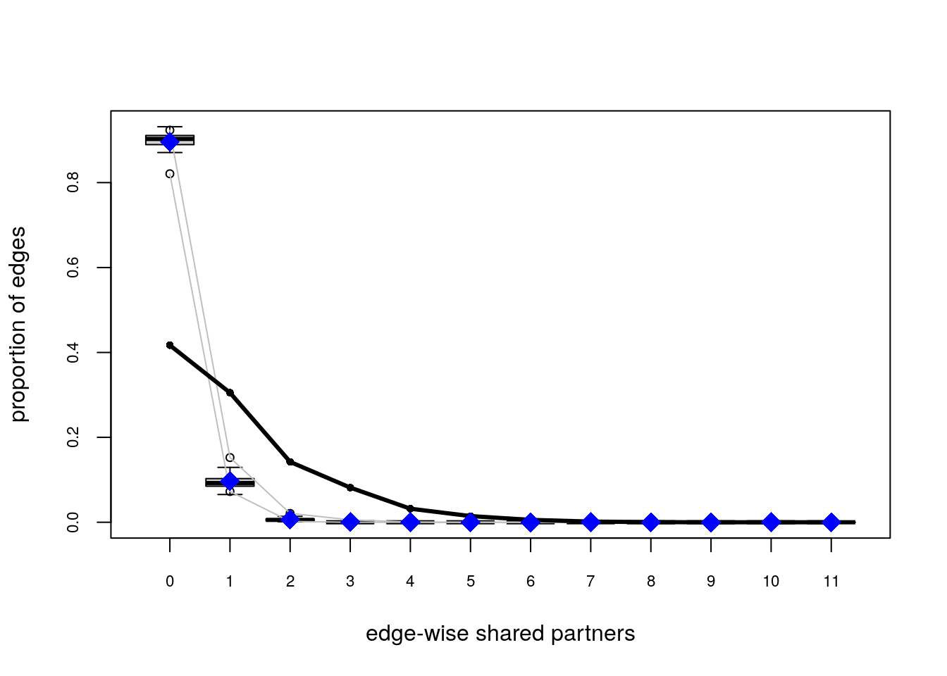
## Goodness-of-fit for edgewise shared partner
##
## obs min mean max MC p-value
## .OTP0 1032 932 1010.98 1087 0.60
## .OTP1 755 690 800.77 908 0.34
## .OTP2 352 318 394.89 464 0.10
## .OTP3 202 112 152.00 201 0.00
## .OTP4 79 24 47.71 81 0.02
## .OTP5 36 2 12.00 24 0.00
## .OTP6 14 0 3.72 18 0.06
## .OTP7 4 0 0.91 6 0.10
## .OTP8 1 0 0.06 2 0.10
## .OTP9 0 0 0.01 1 1.00
# Plotting GOF statistics
plot(ans_gof)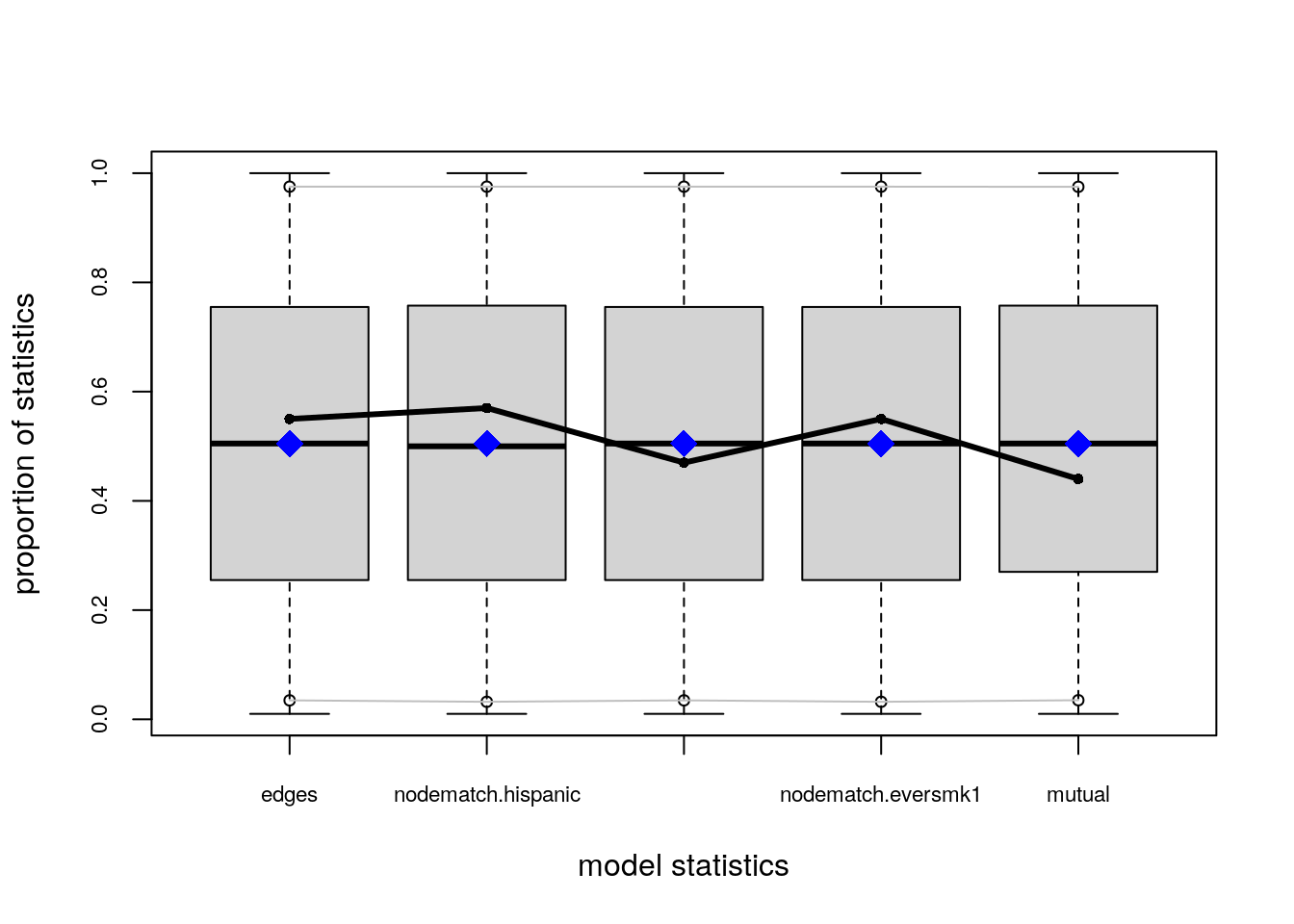
Try the following configuration instead
ans0_bis <- ergm(
  network_111 ~
    edges +
    nodematch("hispanic") +
    nodematch("female1") +
    mutual +
    esp(0:3) +
    idegree(0:10)
    ,
  control = control.ergm(
    seed        = 1,
    MCMLE.maxit = 15,
    parallel    = 4,
    CD.maxit    = 15,
    MCMC.samplesize = 2048*4,
    MCMC.burnin = 30000,
    MCMC.interval = 2048*4
    )
  )
Increase the sample size, so the curves are smoother, longer intervals (thinning), which reduces autocorrelation, and a larger burin. All this together to improve the Gelman test statistic. We also added idegree from 0 to 10, and esp from 0 to 3 to explicitly match those statistics in our model.
For more on this issue, I recommend reviewing chapter 1 and chapter 6 from the Handbook of MCMC (Brooks et al. 2011). Both chapters are free to download from the book’s website.
For GOF take a look at section 6 of ERGM 2016 Sunbelt tutorial, and for a more technical review, you can take a look at (David R. Hunter, Goodreau, and Handcock 2008).
One of the most critical parts of statistical modeling is interpreting the results, if not the most important. In the case of ERGMs, a key aspect is based on change statistics. Suppose that we would like to know how likely the tie y_{ij} is to happen, given the rest of the network. We can compute such probabilities using what literature sometimes describes as the Gibbs-sampler.
In particular, the log-odds of the ij tie occurring conditional on the rest of the network can be written as:
\begin{equation} \text{logit}\left({\Pr{y_{ij} = 1|y_{-ij}}}\right) = {\theta}^\mathbf{t}\Delta\delta\left(y_{ij}:0\to 1\right), \end{equation}
with \delta\left(y_{ij}:0\to 1\right)\equiv s\left(\mathbf{y}\right)_{\text{ij}}^+ - s\left(\mathbf{y}\right)_{\text{ij}}^- as the vector of change statistics, in other words, the difference between the sufficient statistics when y_{ij}=1 and its value when y_{ij} = 0. To show this, we write the following:
\begin{align*} \Pr{y_{ij} = 1|y_{-ij}} & = % \frac{\Pr{y_{ij} = 1, y_{-ij}}}{% {\mathbb{P}_{+}\left(y_{ij} = 1, y_{-ij}\right) } \Pr{y_{ij} = 0, y_{-ij}}} \\ & = \frac{\text{exp}\left\{{\theta}^\mathbf{t}s\left(\mathbf{y}\right)^+_{ij}\right\}}{% \text{exp}\left\{{\theta}^\mathbf{t}s\left(\mathbf{y}\right)^+_{ij}\right\} + \text{exp}\left\{{\theta}^\mathbf{t}s\left(\mathbf{y}\right)^-_{ij}\right\}} \end{align*}
Applying the logit function to the previous equation, we obtain:
\begin{align*} & = \text{log}\left\{\frac{\text{exp}\left\{{\theta}^\mathbf{t}s\left(\mathbf{y}\right)^+_{ij}\right\}}{% \text{exp}\left\{{\theta}^\mathbf{t}s\left(\mathbf{y}\right)^+_{ij}\right\} + % \text{exp}\left\{{\theta}^\mathbf{t}s\left(\mathbf{y}\right)^-_{ij}\right\}}\right\} - % \text{log}\left\{ % \frac{\text{exp}\left\{{\theta}^\mathbf{t}s\left(\mathbf{y}\right)^-_{ij}\right\}}{% \text{exp}\left\{{\theta}^\mathbf{t}s\left(\mathbf{y}\right)^+_{ij}\right\} + \text{exp}\left\{{\theta}^\mathbf{t}s\left(\mathbf{y}\right)^-_{ij}\right\}}% \right\} \\ & = \text{log}\left\{\text{exp}\left\{{\theta}^\mathbf{t}s\left(\mathbf{y}\right)^+_{ij}\right\}\right\} - \text{log}\left\{\text{exp}\left\{{\theta}^\mathbf{t}s\left(\mathbf{y}\right)^-_{ij}\right\}\right\} \\ & = {\theta}^\mathbf{t}\left(s\left(\mathbf{y}\right)^+_{ij} - s\left(\mathbf{y}\right)^-_{ij}\right) \\ & = {\theta}^\mathbf{t}\Delta\delta\left(y_{ij}:0\to 1\right) \end{align*} Therefore, the conditional probability of the tie y_{ij} occurring can be written as:
\begin{equation} {\mathbb{P}_{=}\left(y_{ij} = 1|y_{-ij}\right) } \frac{1}{1 + \text{exp}\left\{-{\theta}^\mathbf{t}\Delta\delta\left(y_{ij}:0\to 1\right)\right\}} \end{equation}
i.e., a logistic probability.
The challenge of analyzing networks is their interdependent nature. Nonetheless, in the absence of such interdependence, ERGMs are equivalent to logistic regression. Conceptually, if all the statistics included in the model do not involve two or more dyads, then the model is dyadic independent.
Mathematically, to see this, it suffices to show that the ERGM probability can be written as the product of each dyads’ individual probabilities.
{\mathbb{P}_{=}\left(\mathbf{y} | \theta\right) } \frac{\text{exp}\left\{{\theta}^\mathbf{t}s\left(\mathbf{y}\right)\right\}}{\sum_{y}\text{exp}\left\{{\theta}^\mathbf{t}s\left(\mathbf{y}\right)\right\}} = \frac{\prod_{ij}\text{exp}\left\{{\theta}^\mathbf{t}s\left(\mathbf{y}\right)_{ij}\right\}}{\sum_{y}\text{exp}\left\{{\theta}^\mathbf{t}s\left(\mathbf{y}\right)\right\}}
Where s\left(\right)_{ij} is a function such that s\left(\mathbf{y}\right) = \sum_{ij}{s\left(\mathbf{y}\right)_{ij}}. We now need to deal with the normalizing constant. The key lies in the fact that we can swap the sum and the product operators. In the case of the dyadic independent model, the normalizing constant can be written as:
\sum_{y\in\mathcal{Y}}\text{exp}\left\{{\theta}^\mathbf{t}s\left(\mathbf{y}\right)\right\} = % \sum_{y\in\mathcal{Y}}\prod_{ij}\text{exp}\left\{{\theta}^\mathbf{t}s\left(\mathbf{y}\right)_{ij}\right\} = % \prod_{ij}\sum_{y\in\{0,1\}}\text{exp}\left\{{\theta}^\mathbf{t}s\left(\mathbf{y}_{ij}\right)\right\}
This can only be achieved with dyadic independence. Otherwise, this arrangement cannot be done. Now, we can write the ERGM model as follows:
\prod_{ij}\left[\frac{% \text{exp}\left\{{\theta}^\mathbf{t}s\left(\mathbf{y}\right)_{ij}\right\}% }{% \sum_{y'\in\{0,1\}}\text{exp}\left\{{\theta}^\mathbf{t}s\left(\mathbf{y}\right)_{ij}\right\}% }\right] = % \prod_{ij}\left[\frac{1}{% 1 + \text{exp}\left\{-{\theta}^\mathbf{t}\Delta\delta\left(y_{ij}:0\to 1\right)\right\}}% \right]
Where the last equality comes from dividing each by the ij-th numerator. Since at least one of the two elements of the \sum_{y'\in\{0,1\}} matches the observed y_{ij}, one reduces to one, and the other to the change statistic.
Related to this, block-diagonal ERGMs can be estimated as independent models, one per block. To see more about this, read (SNIJDERS 2010). Likewise, since independence depends–pun intended–on partitioning the objective function, as pointed by Snijders, non-linear functions make the model dependent, e.g., s\left(\mathbf{y}\right) = \sqrt{\sum_{ij}y_{ij}}, the square root of the edgecount is no longer a bernoulli graph.