Power calculation in network studies

In survey and study design, calculating the required sample size is critical. Nowadays, tools and methods for calculating the required sample size abound; nonetheless, sample size calculation for studies involving social networks is still underdeveloped. This chapter will illustrate how we can use computer simulations to estimate the required sample size. Chapter (part2-power?) provides a general overview of power analysis.

Example 1: Spillover effects in egocentric studies¹

Suppose we want to run an intervention over a particular population, and we are interested in the effects of such intervention on the egos’ alters. In economics, this problem, which they call the “spillover effect,” is actively studied.

We assume that alters only get exposed if egos acquire the behavior for the power calculation. Furthermore, for this first run, we will assume that there is no social reinforcement or influence between alters. We will later relax this assumption. To calculate power, we will do the following:

Simulate egos’ behavior following a logit distribution.
Randomly drop some egos as a result of attrition.
Simulate alters’ behavior using their egos as the treatment.
Fit a logistic regression based on the previous model.
Accept/reject the null and store the result.

The previous steps will be repeated 500 for each value of \(n\) we analyze. We will finalize by plotting power against sample sizes. Let’s first start by writing down the simulation parameters:

# Design
n_sims    <- 500 # Number of simulations
n_a       <- 4   # Number of alters
sizes     <-     # Sizes to try
  seq(from = 100, to = 200, by = 25)

# Assumptions
odds_h_1  <- 2.0 # Odds of Increase/
attrition <- .3
baseline  <- .2  # Low prevalence in 1s

# Parameters
alpha    <- .05
beta_pow <- 0.2

As we discuss in (part2-power?), it is always a good idea to encapsulate the simulation into a function:

# The odds turned to a prob
theta_h_1 <- plogis(log(odds_h_1))

# Simulation function
sim_data <- function(n) {

  # Treatment assignment
  tr  <- c(rep(1, n/2), rep(0, n/2))

  # Step 1: Sampling population of egos
  y_ego <- runif(n) < c(
    rep(theta_h_1, n/2),
    rep(0.5, n/2)
  )

  # Step 2: Simulating attrition
  todrop <- order(runif(n))[1:(n * attrition)]
  y_ego  <- y_ego[-todrop]
  tr     <- tr[-todrop]
  n      <- n - length(todrop)

  # Step 3: Simulating alter's effect. We assume the same as in
  # ego
  tr_alter <- rep(y_ego * tr, n_a)
  y_alter  <- runif(n * n_a) < ifelse(tr_alter, theta_h_1, 0.5)

  # Step 4: Computing test statistic
  res_ego   <- tryCatch(glm(y_ego ~ tr, family = binomial("logit")), error = function(e) e)
  res_alter <- tryCatch(glm(y_alter ~ tr_alter, family = binomial("logit")), error = function(e) e)

  if (inherits(res_ego, "error") | inherits(res_alter, "error"))
    return(c(ego =  NA, alter = NA))
  
  # Step 5: Reject?
  c(
    ego   = summary(res_ego)$coefficients["tr", "Pr(>|z|)"] < alpha,
    alter = summary(res_alter)$coefficients["tr_alter", "Pr(>|z|)"] < alpha
  )
  

}

Now that we have the data generating function, we can run the simulations to approximate statistical power given the sample size. The results will be stored in the matrix spower. Since we are simulating data, it is crucial to set the seed so we can reproduce the results.

# We always set the seed
set.seed(88) 

# Making space, and running!
spower <- NULL
for (s in sizes) {

  # Run the simulation for size s
  simres <- rowMeans(replicate(n_sims, sim_data(s)), na.rm = TRUE)

  # And store the results
  spower <- rbind(spower, simres)

}

The following figure shows the approximate power for finding effects at both levels, ego and alter:

library(ggplot2)

spower <- rbind(
  data.frame(size = sizes, power = spower[,"ego"], type =  "ego"),
  data.frame(size = sizes, power = spower[,"alter"], type =  "alter")
)

spower |>
  ggplot(aes(x = size, y = power, colour = type)) +
  geom_point() +
  geom_smooth(method = "loess", formula = y ~ x) +
  labs(x = "Number of Egos", y = "Approx. Power", colour = "Node type") +
  geom_hline(yintercept = 1 - beta_pow)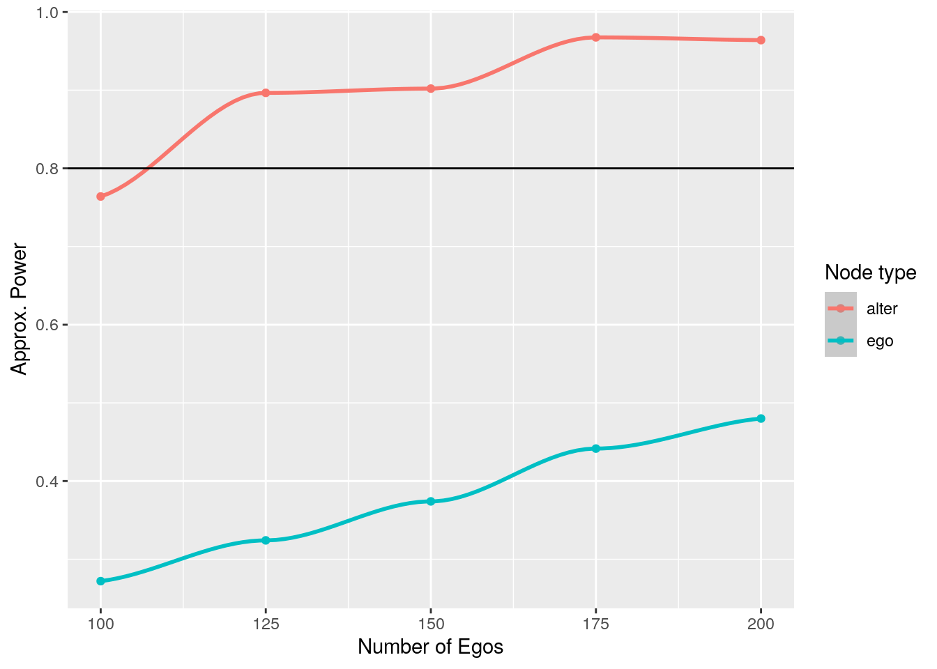

As shown in Chapter (part2-power?), we can use a linear regression model to predict sample size as a function of statistical power:

# Fitting the model
power_model <- glm(
  size ~ power + I(power^2),
  data = spower, family = gaussian(), subset = type == "alter"
)

summary(power_model)


Call:
glm(formula = size ~ power + I(power^2), family = gaussian(), 
    data = spower, subset = type == "alter")

Coefficients:
            Estimate Std. Error t value Pr(>|t|)
(Intercept)     1460       1342   1.088    0.390
power          -3532       3124  -1.131    0.376
I(power^2)      2293       1805   1.270    0.332

(Dispersion parameter for gaussian family taken to be 317.0856)

    Null deviance: 6250.00  on 4  degrees of freedom
Residual deviance:  634.17  on 2  degrees of freedom
AIC: 46.404

Number of Fisher Scoring iterations: 2

# Predict
predict(power_model, newdata = data.frame(power = .8), type = "response") |>
  ceiling()

  1 
102

From the figure, it becomes apparent that, although there is not enough power to identify effects at the ego level, because each ego brings in five alters, the alter sample size is high enough that we can reach above 0.8 statistical power with relatively small sample size.

Example 2: Spillover effects pre-post effect

Now the dynamics are different. Instead of having a treated and control group, we have a single group over which we will measure behavioral change. We will simulate individuals in their initial state, still 0/1, and then simulate that the intervention will make them more likely to have \(y = 1.\) We will also assume that subjects generally don’t change their behavior and that the baseline prevalence of zeros is higher. The simulation steps are as follows:

For each individual in the population, draw the underlying probability that \(y = 1\). With that probability, assign the value of \(y\). This applies to both ego and alter.
Randomly drop some egos, and their corresponding alters due to attrition.
Simulate alters’ behavior using their egos as the treatment. Both ego and alter’s underlying probability are increased by the chosen odds.
To control for the underlying probability that an individual has \(y = 1\), we use conditional logistic regression (also known as matched case-control logit,) to estimate the treatment effects.
Accept/reject the null and store the result.

beta_pars <- c(4, 6)
odds_h_1  <- 2.0

# Simulation function
library(survival)
sim_data_prepost <- function(n) {


  # Step 1: Sampling population of egos
  y_ego_star <- rbeta(n, beta_pars[1], beta_pars[2])
  y_ego_0    <- runif(n) < y_ego_star

  # Step 2: Simulating attrition
  todrop     <- order(runif(n))[1:(n * attrition)]
  y_ego_0    <- y_ego_0[-todrop]
  n          <- n - length(todrop)
  y_ego_star <- y_ego_star[-todrop]

  # Step 3: Simulating alter's effect. We assume the same as in
  # ego
  y_alter_star <- rbeta(n * n_a, beta_pars[1], beta_pars[2])
  y_alter_0    <- runif(n * n_a) < y_alter_star

  # Simulating post
  y_ego_1   <- runif(n) < plogis(qlogis(y_ego_star) + log(odds_h_1))
  tr_alter  <- as.integer(rep(y_ego_1, n_a))
  y_alter_1 <- runif(n * n_a) < plogis(qlogis(y_alter_star) + log(odds_h_1) * tr_alter) # So only if ego did something

  # Step 4: Computing test statistic
  y_ego_0 <- as.integer(y_ego_0)
  y_ego_1 <- as.integer(y_ego_1)
  y_alter_0 <- as.integer(y_alter_0)
  y_alter_1 <- as.integer(y_alter_1)

  d <- data.frame(
    y  = c(y_ego_0, y_ego_1),
    tr = c(rep(0, n), rep(1, n)),
    g  = c(1:n, 1:n)
  )

  res_ego   <- tryCatch(
    clogit(y ~ tr + strata(g), data = d, method = "exact"),
    error = function(e) e
    )

  d <- data.frame(
    y  = c(y_alter_0, y_alter_1),
    tr = c(rep(0, n * n_a), tr_alter),
    g  = c(1:(n * n_a), 1:(n * n_a))
  )

  res_alter <- tryCatch(
    clogit(y ~ tr + strata(g), data = d, method = "exact"),
    error = function(e) e
    )

  if (inherits(res_ego, "error") | inherits(res_alter, "error"))
    return(c(ego =  NA, alter = NA))
  
  # Step 5: Reject?
  c(
    # ego        = res_ego$p.value < alpha,
    ego        = summary(res_ego)$coefficients["tr", "Pr(>|z|)"] < alpha,
    alter      = summary(res_alter)$coefficients["tr", "Pr(>|z|)"] < alpha,
    ego_test   = coef(res_ego),
    alter_glm  = coef(res_alter)
  )
  

}

# We always set the seed 
set.seed(88)

# Making space and running!
spower <- NULL
for (s in sizes) {

  # Run the simulation for size s
  simres <- rowMeans(
    replicate(n_sims, sim_data_prepost(s)),
    na.rm = TRUE
    )

  # And store the results
  spower <- rbind(spower, simres)

}

library(ggplot2)

spowerd <- rbind(
  data.frame(size = sizes, power = spower[,"ego"], type =  "ego"),
  data.frame(size = sizes, power = spower[,"alter"], type =  "alter")
)

spowerd |>
  ggplot(aes(x = size, y = power, colour = type)) +
  geom_point() +
  geom_smooth(method = "loess", formula = y ~ x) +
  labs(x = "Number of Egos", y = "Approx. Power", colour = "Node type") +
  geom_hline(yintercept = 1 - beta_pow)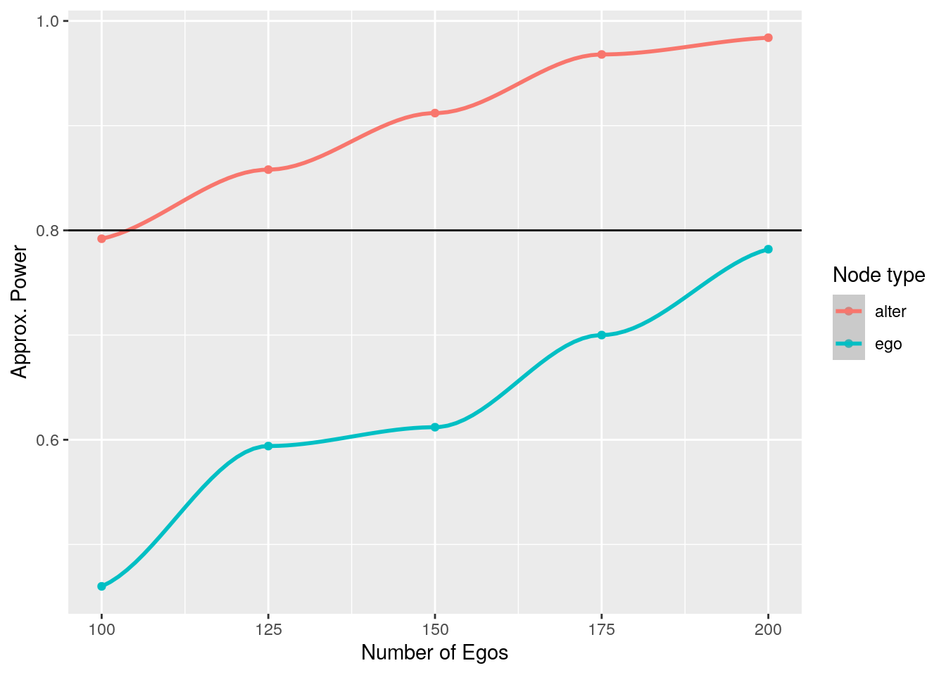

As shown in Chapter (part2-power?), we can use a linear regression model to predict sample size as a function of statistical power:

# Fitting the model
power_model <- glm(
  size ~ power + I(power^2),
  data = spowerd, family = gaussian(), subset = type == "alter"
)

summary(power_model)


Call:
glm(formula = size ~ power + I(power^2), family = gaussian(), 
    data = spowerd, subset = type == "alter")

Coefficients:
            Estimate Std. Error t value Pr(>|t|)
(Intercept)    611.4      666.3   0.918    0.456
power        -1553.8     1504.7  -1.033    0.410
I(power^2)    1147.9      844.8   1.359    0.307

(Dispersion parameter for gaussian family taken to be 52.1536)

    Null deviance: 6250.00  on 4  degrees of freedom
Residual deviance:  104.31  on 2  degrees of freedom
AIC: 37.379

Number of Fisher Scoring iterations: 2

# Predict
predict(power_model, newdata = data.frame(power = .8), type = "response") |>
  ceiling()

  1 
104

Example 3: First difference

Now, instead of looking at a dichotomous outcome, let’s evaluate what happens if the variable is continuous. The effects we are interested to identify are the ego and alter effect, \(\gamma_{ego}\) and \(\gamma_{alter}\), respectively. Furthermore, the data generating process is

\[\begin{align*} y_{itg} & = \alpha_i + \kappa_g + X_i\beta + \varepsilon_{itg} \\ y_{itg} & = \alpha_i + \kappa_g + X_i\beta + D_{i}^{ego}\gamma_{ego} + D_i^{alter}\gamma_{alter} + \varepsilon_{itg} \end{align*}\]

Where \(D_i^{ego/alter}\) is an indicator variable. Here, ego and alter behavior are correlated through a fixed effect. In other words, within each group, we are assuming that there’s a shared baseline prevalence of the outcome. The main difference is that ego and alter may have different results regarding the effect size of the treatment. Another way of approaching the group-level correlation could be through an autocorrelation process, like in a spatial Autocorrelated model; nonetheless, estimating such models is computationally expensive, so we opted to use the former.

For simplicity, we assume that there is no time effect. Two essential components here, \(\alpha_i\) and \(\kappa_g\) are individual and group-level unobserved fixed effects. The most straightforward approach here is to use a first difference estimator:

\[ (y_{it+1g} - y_{itg}) = D_{i}^{ego}\gamma_{ego} + D_i^{alter}\gamma_{alter} + \varepsilon'_i, \quad \varepsilon'_i = \varepsilon_{it+1g} - \varepsilon_{itg} \]

By taking the first difference, the fixed effects are removed from the equation, and we can proceed with a regular linear model.

effect_size_ego   <- 0.5
effect_size_alter <- 0.25
sizes <- seq(10, 100, by = 10)

# Simulation function
sim_data_prepost <- function(n) {

  # Applying attrition
  n <- floor(n * (1 - attrition))

  # Step 1: Sampling fixed effects
  alpha_i <- rnorm(n * (n_a + 1))
  kappa_g <- rep(rnorm(n_a + 1), n)

  # Step 2: Generating the outcome at t = 1
  is_ego   <- rep(c(1, rep(0, n_a)), n)
  is_alter <- 1 - is_ego
  y_0      <- alpha_i + kappa_g + rnorm(n * (n_a + 1))
  y_1      <- alpha_i + kappa_g +
    is_ego * effect_size_ego +
    is_alter * effect_size_alter + 
    rnorm(n * (n_a + 1)) 

  # Step 4: Computing test statistic
  res <- tryCatch(
    glm(I(y_1 - y_0) ~ -1 + is_ego + is_alter, family = gaussian("identity")),
    error = function(e) e
  )

  if (inherits(res, "error"))
    return(c(ego =  NA, alter = NA))
  
  # Step 5: Reject?
  c(
    # ego      = res_ego$p.value < alpha,
    ego        = summary(res)$coefficients["is_ego", "Pr(>|t|)"] < alpha,
    alter      = summary(res)$coefficients["is_alter", "Pr(>|t|)"] < alpha,
    coef(res)[1],
    coef(res)[2]
  )
  

}

# We always set the seed 
set.seed(88)

# Making space and running!
spower <- NULL
for (s in sizes) {

  # Run the simulation for size s
  simres <- rowMeans(
    replicate(n_sims, sim_data_prepost(s)),
    na.rm = TRUE
    )

  # And store the results
  spower <- rbind(spower, simres)

}

library(ggplot2)

spowerd <- rbind(
  data.frame(size = sizes, power = spower[,"ego"], type =  "ego"),
  data.frame(size = sizes, power = spower[,"alter"], type =  "alter")
)

spowerd |>
  ggplot(aes(x = size, y = power, colour = type)) +
  geom_point() +
  geom_smooth(method = "loess", formula = y ~ x) +
  labs(x = "Number of Egos", y = "Approx. Power", colour = "Node type") +
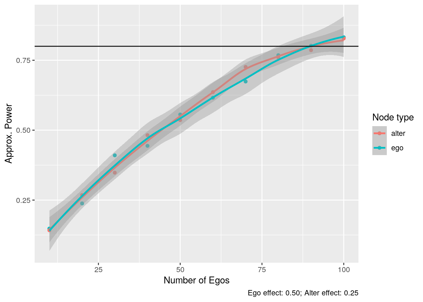
  geom_hline(yintercept = 1 - beta_pow) +
  labs(
    caption = sprintf(
      "Ego effect: %.2f; Alter effect: %.2f", effect_size_ego, effect_size_alter)
      )

From the inferential point of view, we could still use a demean operator to estimate individual-level effects. In particular, we would require to use the demean operator at the group level and then fit a fixed effect model to estimate individual-level parameters.

The original problem was posed by Dr. Shinduk Lee from the School of Nursing at the University of Utah.↩︎

Example 1: Spillover effects in egocentric studies1

Example 2: Spillover effects pre-post effect

Example 3: First difference

Example 1: Spillover effects in egocentric studies¹