This chapter provides a start-to-finish example for processing survey-type data in R. The chapter features the Social Network Study [SNS] dataset. You can download the data for this chapter here, and the codebook for the data provided here is in the appendix.
The goals for this chapter are:
Read the data into R.
Create a network with it.
Compute descriptive statistics.
Visualize the network.
Data preprocessing
Reading the data into R
R has several ways of reading data. Your data can be Raw plain files like CSV, tab-delimited, or specified by column width. To read plain-text data, you can use the readr package (Wickham, Hester, and Bryan 2024). In the case of binary files, like Stata, Octave, or SPSS files, you can use the R package foreign(R Core Team 2023). If your data is formatted as Microsoft spreadsheets, the readxl R package (Wickham and Bryan 2023) is the alternative to use. In our case, the data for this session is in Stata format:
library(foreign)# Reading the datadat <- foreign::read.dta("03-sns.dta")# Taking a look at the data's first 5 columns and 5 rowsdat[1:5, 1:10]
  photoid school hispanic female1 female2 female3 female4 grades1 grades2
1       1    111        1      NA      NA       0       0      NA      NA
2       2    111        1       0      NA      NA       0     3.0      NA
3       7    111        0       1       1       1       1     5.0     4.5
4      13    111        1       1       1       1       1     2.5     2.5
5      14    111        1       1       1       1      NA     3.0     3.5
  grades3
1     3.5
2      NA
3     4.0
4     2.5
5     3.5
Creating a unique id for each participant
We must create a unique id using the school and photo id. Since both variables are numeric, encoding the id is a good way of doing this. For example, the last three numbers are the photoid, and the first numbers are the school id. To do this, we need to take into account the range of the variables:
(photo_id_ran <-range(dat$photoid))
[1] 1 2074
As the variable spans up to 2074, we need to set the last 4 units of the variable to store the photoid. We will use dplyr(Wickham et al. 2023) to create this variable and call it id:
library(dplyr)
Attaching package: 'dplyr'
The following objects are masked from 'package:stats':

    filter, lag
The following objects are masked from 'package:base':

    intersect, setdiff, setequal, union
# Creating the variabledat <- dat |>mutate(id = school*10000+ photoid)# First few rowsdat |>head() |>select(school, photoid, id)
Wow, what happened in the last lines of code?! What is that |>? Well, that’s the pipe operator1, and it is an appealing way of writing nested function calls. In this case, instead of writing something like:
We want to build a social network. For that, we either use an adjacency matrix or an edgelist.
Each individual of the SNS data nominated 19 friends from school. We will use those nominations to create the social network.
In this case, we will create the network by coercing the dataset into an edgelist.
From survey to edgelist
Let’s start by loading a couple of handy R packages. We will load tidyr(Wickham, Vaughan, and Girlich 2024) and stringr(Wickham 2023). We will use the first, tidyr, to reshape the data. The second, stringr, will help us processing strings using regular expressions2.
library(tidyr)library(stringr)
Optionally, we can use the tibble type of object, an alternative to the actual data.frame. This object provides more efficient methods for matrices and data frames.
dat <-as_tibble(dat)
What I like about tibbles is that when you print them on the console, these look nice:
dat
# A tibble: 2,164 × 100
   photoid school hispanic female1 female2 female3 female4 grades1 grades2
     <int>  <int>    <dbl>   <int>   <int>   <int>   <int>   <dbl>   <dbl>
 1       1    111        1      NA      NA       0       0    NA      NA
 2       2    111        1       0      NA      NA       0     3      NA
 3       7    111        0       1       1       1       1     5       4.5
 4      13    111        1       1       1       1       1     2.5     2.5
 5      14    111        1       1       1       1      NA     3       3.5
 6      15    111        1       0       0       0       0     2.5     2.5
 7      20    111        1       1       1       1       1     2.5     2.5
 8      22    111        1      NA      NA       0       0    NA      NA
 9      25    111        0       1       1      NA       1     4.5     3.5
10      27    111        1       0      NA       0       0     3.5    NA
# ℹ 2,154 more rows
# ℹ 91 more variables: grades3 <dbl>, grades4 <dbl>, eversmk1 <int>,
#   eversmk2 <int>, eversmk3 <int>, eversmk4 <int>, everdrk1 <int>,
#   everdrk2 <int>, everdrk3 <int>, everdrk4 <int>, home1 <int>, home2 <int>,
#   home3 <int>, home4 <int>, sch_friend11 <int>, sch_friend12 <int>,
#   sch_friend13 <int>, sch_friend14 <int>, sch_friend15 <int>,
#   sch_friend16 <int>, sch_friend17 <int>, sch_friend18 <int>, …
# Maybe too much piping... but its cool!net <- dat |>select(id, school, starts_with("sch_friend")) |>gather(key ="varname", value ="content", -id, -school) |>filter(!is.na(content)) |>mutate(friendid = school*10000+ content,year =as.integer(str_extract(varname, "(?<=[a-z])[0-9]")),nnom =as.integer(str_extract(varname, "(?<=[a-z][0-9])[0-9]+")) )
Let’s take a look at this step by step:
First, we subset the data: We want to keep id, school, sch_friend*. For the latter, we use the function starts_with (from the tidyselect package). The latter allows us to select all variables that start with the word “sch_friend”, which means that sch_friend11, sch_friend12, ... will be selected.
dat |>select(id, school, starts_with("sch_friend"))
# A tibble: 2,164 × 78
        id school sch_friend11 sch_friend12 sch_friend13 sch_friend14
     <dbl>  <int>        <int>        <int>        <int>        <int>
 1 1110001    111           NA           NA           NA           NA
 2 1110002    111          424          423          426          289
 3 1110007    111          629          505           NA           NA
 4 1110013    111          232          569           NA           NA
 5 1110014    111          582          134           41          592
 6 1110015    111           26          488           81          138
 7 1110020    111          528           NA          492          395
 8 1110022    111           NA           NA           NA           NA
 9 1110025    111          135          185          553           84
10 1110027    111          346          168          559            5
# ℹ 2,154 more rows
# ℹ 72 more variables: sch_friend15 <int>, sch_friend16 <int>,
#   sch_friend17 <int>, sch_friend18 <int>, sch_friend19 <int>,
#   sch_friend110 <int>, sch_friend111 <int>, sch_friend112 <int>,
#   sch_friend113 <int>, sch_friend114 <int>, sch_friend115 <int>,
#   sch_friend116 <int>, sch_friend117 <int>, sch_friend118 <int>,
#   sch_friend119 <int>, sch_friend21 <int>, sch_friend22 <int>, …
Then, we reshape it to long format: By transposing all the sch_friend* to long format. We do this using the function gather (from the tidyr package); an alternative to the reshape function, which I find easier to use. Let’s see how it works:
dat |>select(id, school, starts_with("sch_friend")) |>gather(key ="varname", value ="content", -id, -school)
In this case, the key parameter sets the name of the variable that will contain the name of the variable that was reshaped, while value is the name of the variable that will hold the content of the data (that’s why I named those like that). The -id, -school bit tells the function to “drop” those variables before reshaping. In other words, “reshape everything but id and school.”
Also, notice that we passed from 2164 rows to 19 (nominations) * 2164 (subjects) * 4 (waves) = 164464 rows, as expected.
As the nomination data can be empty for some cells, we need to take care of those cases, the NAs, so we filter the data:
dat |>select(id, school, starts_with("sch_friend")) |>gather(key ="varname", value ="content", -id, -school) |>filter(!is.na(content))
The regular expression (?<=[a-z]) matches a string preceded by any letter from a to z. In contrast, the expression [0-9] matches a single number. Hence, from the string "sch_friend12", the regular expression will only match the 1, as it is the only number followed by a letter. The expression (?<=[a-z][0-9]) matches a string preceded by a lowercase letter and a one-digit number. Finally, the expression [0-9]+ matches a string of numbers–so it could be more than one. Hence, from the string "sch_friend12", we will get 2:
And finally, the as.integer function coerces the returning value from the str_extract function from character to integer. Now that we have this edgelist, we can create an igraph object
igraph network
For coercing the edgelist into an igraph object, we will be using the graph_from_data_frame function in igraph (Csárdi et al. 2024). This function receives the following arguments: a data frame where the two first columns are “source” (ego) and “target” (alter), an indicator of whether the network is directed or not, and an optional data frame with vertices, in which’s first column should contain the vertex ids.
Using the optional vertices argument is a good practice: It tells the function what ids should expect. Using the original dataset, we will create a data frame with name vertices:
vertex_attrs <- dat |>select(id, school, hispanic, female1, starts_with("eversmk"))
Now, let’s now use the function graph_from_data_frame to create an igraph object:
Error in `graph_from_data_frame()`:
! Some vertex names in `d` are not listed in `vertices`
Ups! It seems that individuals are nominating other students not included in the survey. How to solve that? Well, it all depends on what you need to do! In this case, we will go for the quietly-remove-em’-and-don’t-tell strategy:
library(igraph)ig_year1 <- net |>filter(year =="1") |># Extra line, all nominations must be in ego too.filter(friendid %in% id) |>select(id, friendid, nnom) |>graph_from_data_frame(vertices = vertex_attrs )ig_year1
So we have our network with 2164 nodes and 9514 edges. The following steps: get some descriptive stats and visualize our network.
Network descriptive stats
While we could do all networks at once, in this part, we will focus on computing some network statistics for one of the schools only. We start by school 111. The first question that you should be asking yourself now is, “how can I get that information from the igraph object?.” Vertex and edges attributes can be accessed via the V and E functions, respectively; moreover, we can list what vertex/edge attributes are available:
Just like we would do with data frames, accessing vertex attributes is done via the dollar sign operator $. Together with the V function; for example, accessing the first ten elements of the variable hispanic can be done as follows:
V(ig_year1)$hispanic[1:10]
[1] 1 1 0 1 1 1 1 1 0 1
Now that you know how to access vertex attributes, we can get the network corresponding to school 111 by identifying which vertices are part of it and pass that information to the induced_subgraph function:
# Which ids are from school 111?school111ids <-which(V(ig_year1)$school ==111)# Creating a subgraphig_year1_111 <-induced_subgraph(graph = ig_year1,vids = school111ids)
The which function in R returns a vector of indices indicating which elements pass the test, returning true and false, otherwise. In our case, it will result in a vector of indices of the vertices which have the attribute school equal to 111. With the subgraph, we can compute different centrality measures3 for each vertex and store them in the igraph object itself:
# Computing centrality measures for each vertexV(ig_year1_111)$indegree <-degree(ig_year1_111, mode ="in")V(ig_year1_111)$outdegree <-degree(ig_year1_111, mode ="out")V(ig_year1_111)$closeness <-closeness(ig_year1_111, mode ="total")V(ig_year1_111)$betweeness <-betweenness(ig_year1_111, normalized =TRUE)
From here, we can go back to our old habits and get the set of vertex attributes as a data frame so we can compute some summary statistics on the centrality measurements that we just got
# Extracting each vertex features as a data.framestats <-as_data_frame(ig_year1_111, what ="vertices")# Computing quantiles for each variablestats_degree <-with(stats, {cbind(indegree =quantile(indegree, c(.025, .5, .975), na.rm =TRUE),outdegree =quantile(outdegree, c(.025, .5, .975), na.rm =TRUE),closeness =quantile(closeness, c(.025, .5, .975), na.rm =TRUE),betweeness =quantile(betweeness, c(.025, .5, .975), na.rm =TRUE) )})stats_degree
The with function is somewhat similar to what dplyr allows us to do when we want to work with the dataset but without mentioning its name everytime that we ask for a variable. Without using the with function, the previous could have been done as follows:
To get a nicer view of this, we can use a table that I retrieved from ?triad_census. Moreover, we can normalize the triadic object by its sum instead of looking at raw counts. That way, we get proportions instead4
A<->B, C, the graph with a mutual connection between two vertices.
0.01
021D
A<-B->C, the out-star.
0.01
021U
A->B<-C, the in-star.
0.02
021C
A->B->C, directed line.
0.01
111D
A<->B<-C.
0.01
111U
A<->B->C.
0.00
030T
A->B<-C, A->C.
0.00
030C
A<-B<-C, A->C.
0.00
201
A<->B<->C.
0.00
120D
A<-B->C, A<->C.
0.00
120U
A->B<-C, A<->C.
0.00
120C
A->B->C, A<->C.
0.00
210
A->B<->C, A<->C.
0.00
300
A<->B<->C, A<->C, the complete graph.
Plotting the network in igraph
Single plot
Let’s take a look at how does our network looks like when we use the default parameters in the plot method of the igraph object:
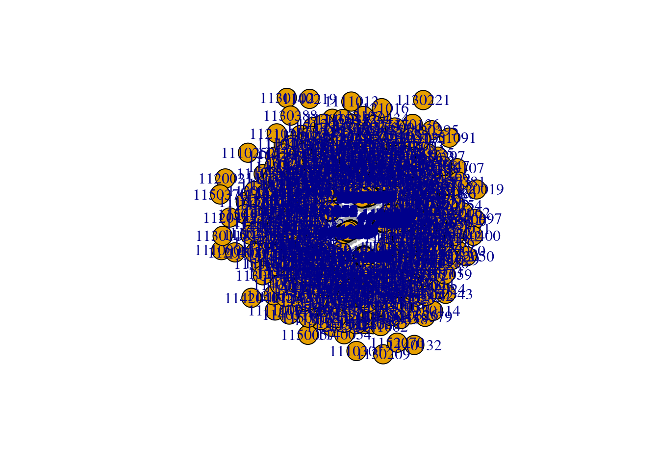
plot(ig_year1)
A not very nice network plot. This is what we get with the default parameters in igraph.
Not very nice, right? A couple of things with this plot:
We are looking at all schools simultaneously, which does not make sense. So, instead of plotting ig_year1, we will focus on ig_year1_111.
All the vertices have the same size and are overlapping. Instead of using the default size, we will size the vertices by indegree using the degree function and passing the vector of degrees to vertex.size.5
Given the number of vertices in these networks, the labels are not useful here. So we will remove them by setting vertex.label = NA. Moreover, we will reduce the size of the arrows’ tip by setting edge.arrow.size = 0.25.
And finally, we will set the color of each vertex to be a function of whether the individual is Hispanic or not. For this last bit we need to go a bit more of programming:
The first line added one to all no NA values so that the 0s (non-Hispanic) turned to 1s and the 1s (Hispanic) turned to 2s.
The second line replaced all NAs with the number three so that our vector col_hispanic now ranges from one to three with no NAs in it.
In the last line, we created a vector of colors. Essentially, what we are doing here is telling R to create a vector of length length(col_hispanic) by selecting elements by index from the vector c("steelblue", "tomato", "white"). This way, if, for example, the first element of the vector col_hispanic was a 3, our new vector of colors would have a "white" in it.
To make sure we know we are right, let’s print the first 10 elements of our new vector of colors together with the original hispanic column:
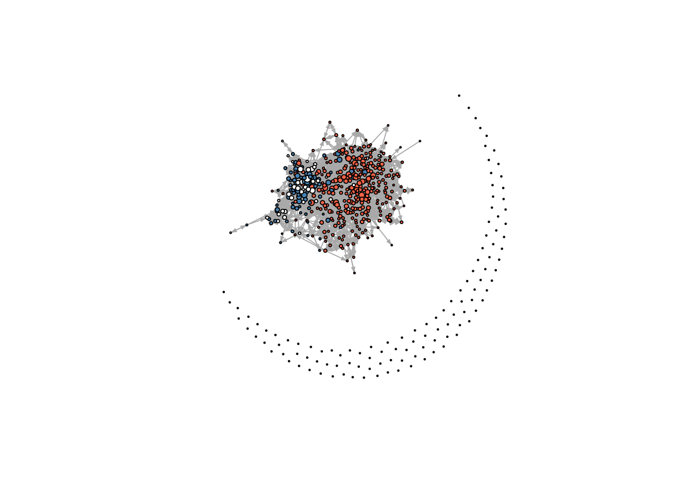
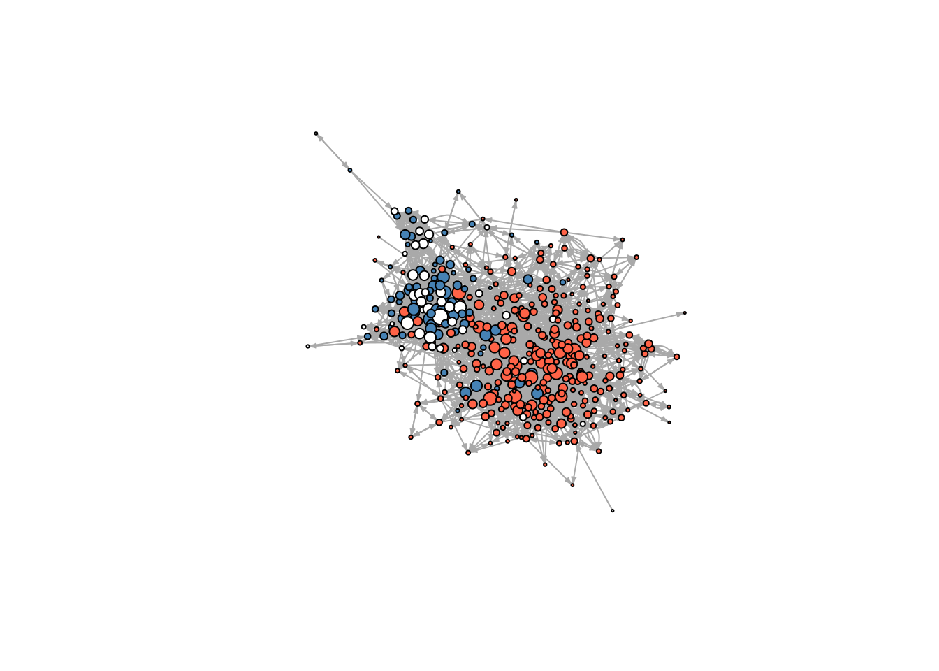
Nice! So it does look better. The only problem is that we have a lot of isolates. Let’s try again by drawing the same plot without isolates. To do so, we need to filter the graph, for which we will use the function induced_subgraph
# Which vertices are not isolates?which_ids <-which(degree(ig_year1_111, mode ="total") >0)# Getting the subgraphig_year1_111_sub <-induced_subgraph(ig_year1_111, which_ids)# We need to get the same subset in col_hispaniccol_hispanic <- col_hispanic[which_ids]
Friends network in time 1 for school 111. The graph excludes isolates.
Now that’s better! An interesting pattern that shows up is that individuals seem to cluster by whether they are Hispanic or not.
We can write this as a function to avoid copying and pasting the code n times (supposing that we want to create a plot similar to this n times). We do the latter in the following subsection.
Multiple plots
When you are repeating yourself repeatedly, it is a good idea to write down a sequence of commands as a function. In this case, since we will be running the same type of plot for all schools/waves, we write a function in which the only things that change are: (a) the school id, and (b) the color of the nodes.
The myplot <- function([arguments]) {[body of the function]} tells R that we are going to create a function called myplot.
We declare four specific arguments: net, schoolid, mindgr, and vcol. These are an igraph object, the school id, the minimum degree that vertices must have to be included in the figure, and the color of the vertices. Observe that, compared to other programming languages, R does not require declaring the data types.
The ellipsis object, ..., is an especial object in R that allows us to pass other arguments without specifying which. If you take a look at the plot bit in the function body, you will see that we also added .... We use the ellipsis to pass extra arguments (different from the ones that we explicitly defined) directly to plot. In practice, this implies that we can, for example, set the argument edge.arrow.size when calling myplot, even though we did not include it in the function definition! (See ?dotsMethods in R for more details).
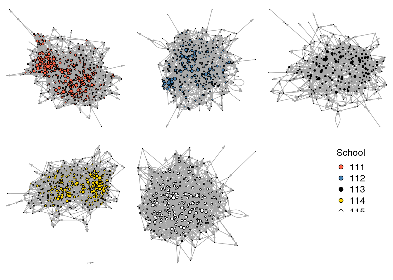
In the following lines of code, using our new function, we will plot each schools’ network in the same plotting device (window) with the help of the par function, and add legend with the legend:
All 5 schools in time 1. Again, the graphs exclude isolates.
So what happened here?
oldpar <- par(no.readonly = TRUE) This line stores the current parameters for plotting. Since we are going to be changing them, we better make sure we are able to go back!.
par(mfrow = c(2, 3), mai = rep(0, 4), oma=rep(0, 4)) Here we are setting various things at the same time. mfrow specifies how many figures will be drawn, and in what order. In particular, we are asking the plotting device to make room for 2*3 = 6 figures organized in two rows and three columns drawn by row.
mai specifies the size of the margins in inches, setting all margins equal to zero (which is what we are doing now) gives more space to the graph. The same is true for oma. See ?par for more info.
myplot(ig_year1, ...) This is simply calling our plotting function. The neat part of this is that, since we set mfrow = c(2, 3), R takes care of distributing the plots in the device.
par(oldpar) This line allows us to restore the plotting parameters.
Statistical tests
Is nomination number correlated with indegree?
Hypothesis: Individuals that, on average, are among the first nominations of their peers are more popular
# Getting all the data in long formatedgelist <-as_long_data_frame(ig_year1) |>as_tibble()# Computing indegree (again) and average nomination number# Include "On a scale from one to five how close do you feel"# Also for egocentric friends (A. Friends)indeg_nom_cor <-group_by(edgelist, to, to_name, to_school) |>summarise(indeg =length(nnom),nom_avg =1/mean(nnom) ) |>rename(school = to_school )
`summarise()` has grouped output by 'to', 'to_name'. You can override using the
`.groups` argument.
# Using pearson's correlationwith(indeg_nom_cor, cor.test(indeg, nom_avg))
    Pearson's product-moment correlation

data:  indeg and nom_avg
t = -12.254, df = 1559, p-value < 2.2e-16
alternative hypothesis: true correlation is not equal to 0
95 percent confidence interval:
 -0.3409964 -0.2504653
sample estimates:
       cor
-0.2963965
save.image("03.rda")
Csárdi, Gábor, Tamás Nepusz, Vincent Traag, Szabolcs Horvát, Fabio Zanini, Daniel Noom, and Kirill Müller. 2024. igraph: Network Analysis and Visualization in r. https://doi.org/10.5281/zenodo.7682609.
Wickham, Hadley, Romain François, Lionel Henry, Kirill Müller, and Davis Vaughan. 2023. Dplyr: A Grammar of Data Manipulation. https://dplyr.tidyverse.org.
Wickham, Hadley, Jim Hester, and Jennifer Bryan. 2024. Readr: Read Rectangular Text Data. https://readr.tidyverse.org.
Wickham, Hadley, Davis Vaughan, and Maximilian Girlich. 2024. Tidyr: Tidy Messy Data. https://tidyr.tidyverse.org.
Please refer to the help file ?'regular expression' in R. The R package rex(Ushey, Hester, and Krzyzanowski 2021) is a friendly companion for writing regular expressions. There’s also a neat (but experimental) RStudio add-in that can be very helpful for understanding how regular expressions work, the regexplain add-in.↩︎
For more information about the different centrality measurements, please take a look at the “Centrality” article on Wikipedia.↩︎
During our workshop, Prof. De la Haye suggested using {n \choose 3} as a normalizing constant. It turns out that sum(triadic) = choose(n, 3)! So either approach is correct.↩︎
Figuring out what is the optimal vertex size is a bit tricky. Without getting too technical, there’s no other way of getting nice vertex size other than just playing with different values of it. A nice solution to this is using netdiffuseR::igraph_vertex_rescale which rescales the vertices so that these keep their aspect ratio to a predefined proportion of the screen.↩︎