This chapter is based on the 2018 and 2019 tutorials of netdiffuseR at the Sunbelt conference. The source code of the tutorials, taught by Thomas W. Valente and George G. Vega Yon (author of this book), is available here.
Network diffusion of innovation
Diffusion networks
Explains how new ideas and practices (innovations) spread within and between communities.
While a lot of factors have been shown to influence diffusion (Spatial, Economic, Cultural, Biological, etc.), Social Networks are prominent.
There are many components in the diffusion network model, including network exposures, thresholds, infectiousness, susceptibility, hazard rates, diffusion rates (bass model), clustering (Moran’s I), and so on.
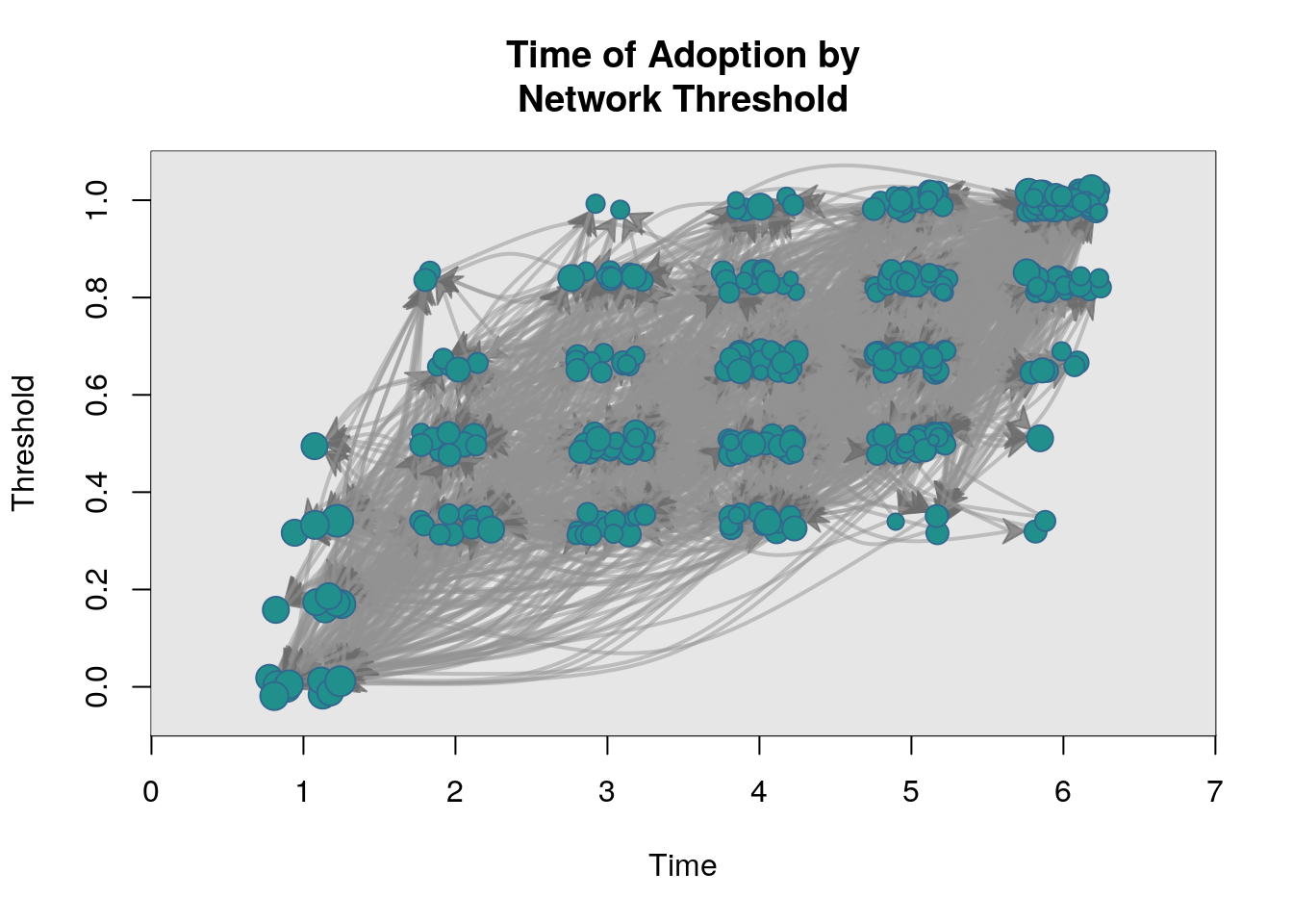
Thresholds
One of the canonical concepts is the network threshold. Network thresholds (Valente, 1995; 1996), \tau, are defined as the required proportion or number of neighbors that lead you to adopt a particular behavior (innovation), a=1. In (very) general terms
Where E_i is i’s exposure to the innovation and \mathbf{X} is the adjacency matrix (the network).
This can be generalized and extended to include covariates and other network weighting schemes (that’s what netdiffuseR is all about).
The netdiffuseR R package
Overview
netdiffuseR is an R package that:
It is designed to Visualize, Analyze, and simulate network diffusion data (in general).
Depends on some pretty popular packages:
RcppArmadillo: So it’s fast,
Matrix: So it’s big,
statnet and igraph: So it’s not from scratch
Can handle big graphs, e.g., an adjacency matrix with more than 4 billion elements (PR for RcppArmadillo)
Already on CRAN with ~6,000 downloads since its first version, Feb 2016,
A lot of features to make it easy to read network (dynamic) data, making it a companion of other net packages.
Datasets
netdiffuseR has the three classic Diffusion Network Datasets:
medInnovationsDiffNet Doctors and the innovation of Tetracycline (1955).
brfarmersDiffNet Brazilian farmers and the innovation of Hybrid Corn Seed (1966).
kfamilyDiffNet Korean women and Family Planning methods (1973).
brfarmersDiffNet
Dynamic network of class -diffnet-
 Name               : Brazilian Farmers
 Behavior           : Adoption of Hybrid Corn Seeds
 # of nodes         : 692 (1001, 1002, 1004, 1005, 1007, 1009, 1010, 1020, ...)
 # of time periods  : 21 (1946 - 1966)
 Type               : directed
 Num of behaviors   : 1
 Final prevalence   : 1.00
 Static attributes  : village, idold, age, liveout, visits, contact, coo... (146)
 Dynamic attributes : -
medInnovationsDiffNet
Dynamic network of class -diffnet-
 Name               : Medical Innovation
 Behavior           : Adoption of Tetracycline
 # of nodes         : 125 (1001, 1002, 1003, 1004, 1005, 1006, 1007, 1008, ...)
 # of time periods  : 18 (1 - 18)
 Type               : directed
 Num of behaviors   : 1
 Final prevalence   : 1.00
 Static attributes  : city, detail, meet, coll, attend, proage, length, ... (58)
 Dynamic attributes : -
kfamilyDiffNet
Dynamic network of class -diffnet-
 Name               : Korean Family Planning
 Behavior           : Family Planning Methods
 # of nodes         : 1047 (10002, 10003, 10005, 10007, 10010, 10011, 10012, 10014, ...)
 # of time periods  : 11 (1 - 11)
 Type               : directed
 Num of behaviors   : 1
 Final prevalence   : 1.00
 Static attributes  : village, recno1, studno1, area1, id1, nmage1, nmag... (430)
 Dynamic attributes : -
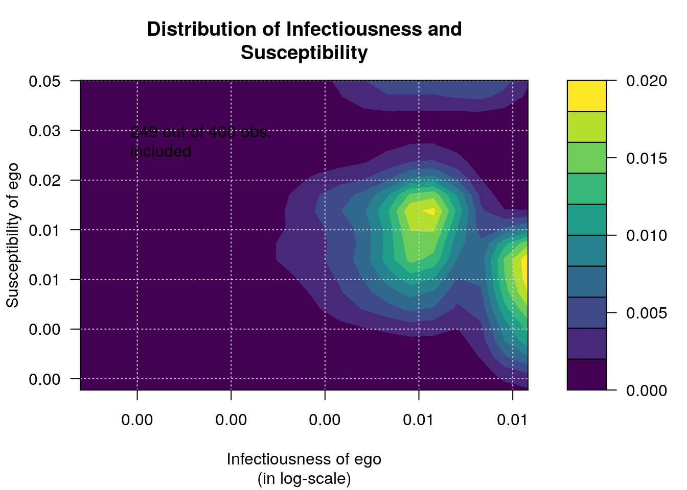
Warning in plot_infectsuscep.list(graph$graph, graph$toa, t0, normalize, : When
applying logscale some observations are missing.
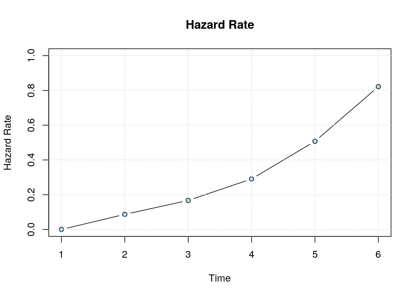
plot_hazard(x)
Problems
Using the diffnet object in intro.rda, use the function plot_threshold specifying shapes and colors according to the variables ItrustMyFriends and Age. Do you see any pattern?
Simulation of diffusion processes
Before we start, a review of the concepts we will be using here
Exposure: Proportion/number of neighbors that have adopted an innovation at each point in time.
Threshold: The proportion/number of your neighbors who had adopted at or one time period before ego (the focal individual) adopted.
Infectiousness: How much i’s adoption affects her alters.
Susceptibility: How much i’s alters’ adoption affects her.
Structural equivalence: How similar is i to j in terms of position in the network.
Simulating diffusion networks
We will simulate a diffusion network with the following parameters:
Will have 1,000 vertices,
Will span 20 time periods,
The initial adopters (seeds) will be selected at random,
Seeds will be a 10% of the network,
The graph (network) will be small-world,
Will use the WS algorithm with p=.2 (probability of rewiring).
Threshold levels will be uniformly distributed between [0.3, 0.7]
To generate this diffusion network, we can use the rdiffnet function included in the package:
# Setting the seed for the RNGset.seed(1213)# Generating a random diffusion networknet <-rdiffnet(n =1e3, # 1.t =20, # 2.seed.nodes ="random", # 3.seed.p.adopt = .1, # 4.seed.graph ="small-world", # 5.rgraph.args =list(p=.2), # 6.threshold.dist =function(x) runif(1, .3, .7) # 7. )
The function rdiffnet generates random diffusion networks. Main features:
Simulating random graph or using your own,
Setting threshold levels per node,
Network rewiring throughout the simulation, and
Setting the seed nodes.
The simulation algorithm is as follows:
If required, a baseline graph is created,
Set of initial adopters and threshold distribution are established,
The set of t networks is created (if required), and
Simulation starts at t=2, assigning adopters based on exposures and thresholds:
For each i \in N, if its exposure at t-1 is greater than its threshold, then adopts, otherwise, continue without change.
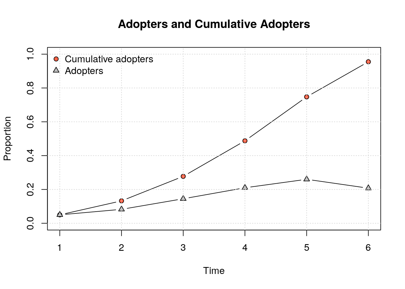
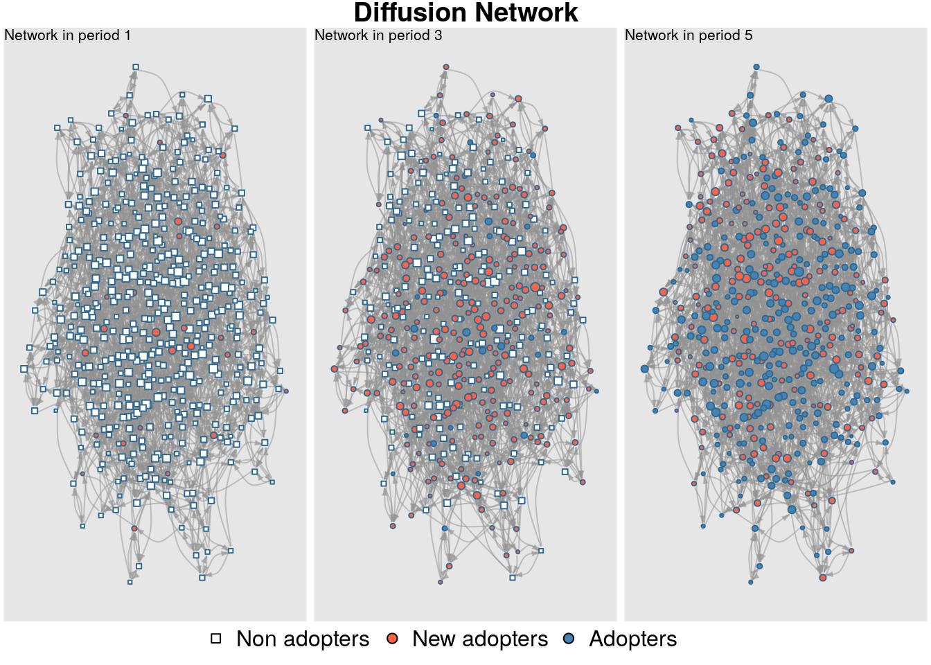
Diffusion network summary statistics
 Name     :  A diffusion network
 Behavior : Random contagion
-----------------------------------------------------------------------------
 Period   Adopters   Cum Adopt. (%)   Hazard Rate   Density   Moran's I (sd)
-------- ---------- ---------------- ------------- --------- ----------------
       1         25        25 (0.05)             -      0.01 -0.00 (0.00)
       2         78       103 (0.21)          0.16      0.01  0.01 (0.00) ***
       3        187       290 (0.58)          0.47      0.01  0.01 (0.00) ***
       4        183       473 (0.95)          0.87      0.01  0.01 (0.00) ***
       5         27       500 (1.00)          1.00      0.01               -
-----------------------------------------------------------------------------
 Left censoring  : 0.05 (25)
 Right centoring : 0.00 (0)
 # of nodes      : 500

 Moran's I was computed on contemporaneous autocorrelation using 1/geodesic
 values. Significane levels  *** <= .01, ** <= .05, * <= .1.
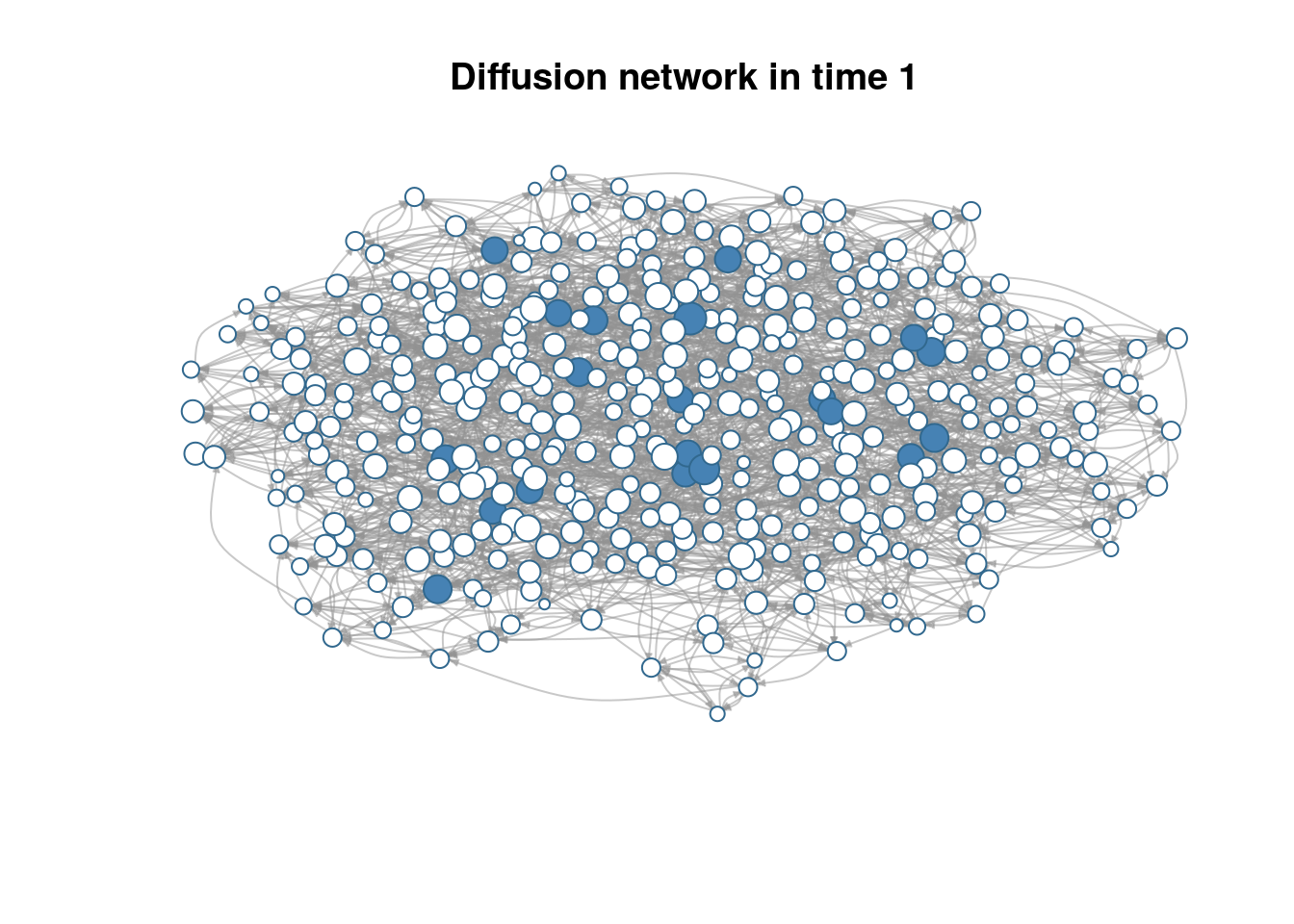
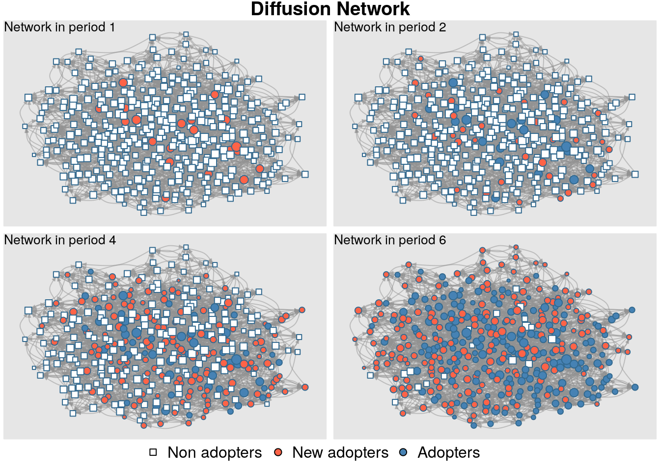
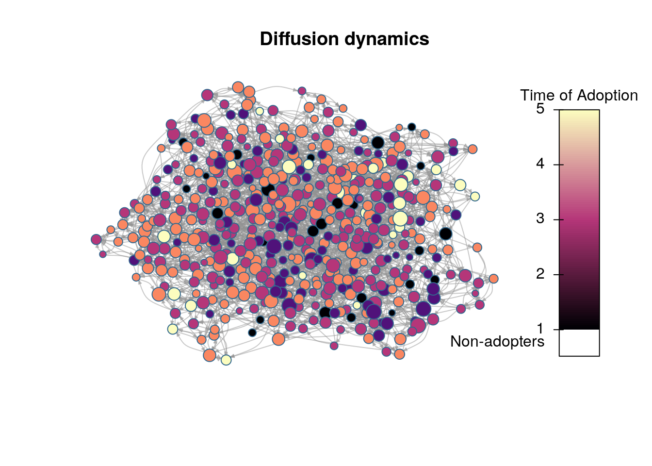
plot_diffnet(diffnet_rumor, slices =c(1, 3, 5))
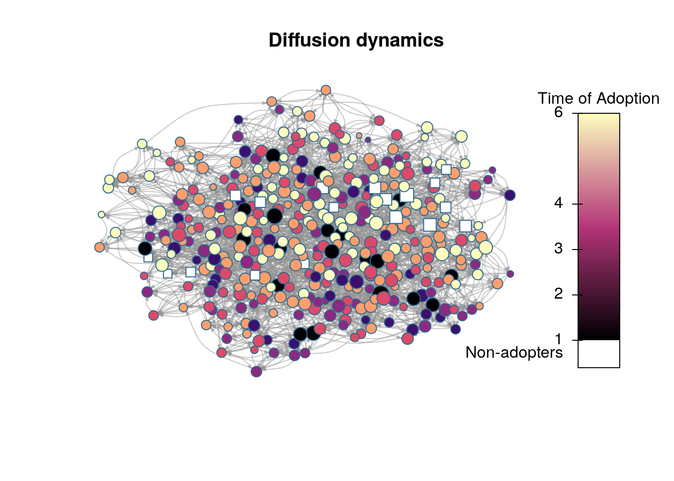
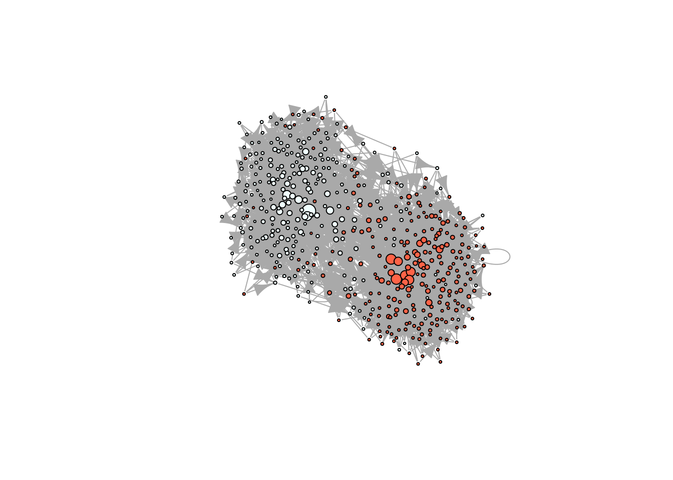
# We want to use igraph to compute layoutigdf <-diffnet_to_igraph(diffnet_rumor, slices=c(1,2))[[1]]pos <- igraph::layout_with_drl(igdf)plot_diffnet2(diffnet_rumor, vertex.size =dgr(diffnet_rumor)[,1], layout=pos)
# Simulating a scale-free homophilic networkset.seed(1231)X <-rep(c(1,1,1,1,1,0,0,0,0,0), 50)net <-rgraph_ba(t =499, m=4, eta = X)# Taking a look in igraphig <- igraph::graph_from_adjacency_matrix(net)plot(ig, vertex.color =c("azure", "tomato")[X+1], vertex.label =NA,vertex.size =sqrt(dgr(net)))
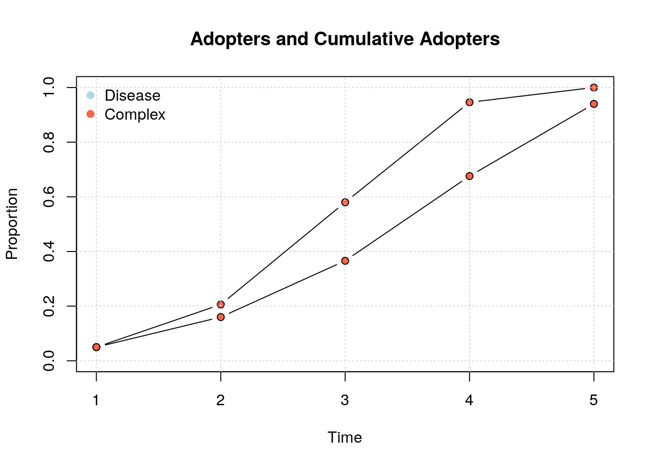
# Now, simulating a bunch of diffusion processesnsim <-500Lans_1and2 <-vector("list", nsim)set.seed(223)for (i in1:nsim) {# We just want the cum adopt count ans_1and2[[i]] <-cumulative_adopt_count(rdiffnet(seed.graph = net,t =10,threshold.dist =sample(1:2, 500L, TRUE),seed.nodes ="random",seed.p.adopt = .10,exposure.args =list(outgoing =FALSE, normalized =FALSE),rewire =FALSE ) )# Are we there yet?if (!(i %%50))message("Simulation ", i," of ", nsim, " done.")}## Simulation 50 of 500 done.## Simulation 100 of 500 done.## Simulation 150 of 500 done.## Simulation 200 of 500 done.## Simulation 250 of 500 done.## Simulation 300 of 500 done.## Simulation 350 of 500 done.## Simulation 400 of 500 done.## Simulation 450 of 500 done.## Simulation 500 of 500 done.# Extracting propans_1and2 <-do.call(rbind, lapply(ans_1and2, "[", i="prop", j=))ans_2and3 <-vector("list", nsim)set.seed(223)for (i in1:nsim) {# We just want the cum adopt count ans_2and3[[i]] <-cumulative_adopt_count(rdiffnet(seed.graph = net,t =10,threshold.dist =sample(2:3, 500L, TRUE),seed.nodes ="random",seed.p.adopt = .10,exposure.args =list(outgoing =FALSE, normalized =FALSE),rewire =FALSE ) )# Are we there yet?if (!(i %%50))message("Simulation ", i," of ", nsim, " done.")}## Simulation 50 of 500 done.## Simulation 100 of 500 done.## Simulation 150 of 500 done.## Simulation 200 of 500 done.## Simulation 250 of 500 done.## Simulation 300 of 500 done.## Simulation 350 of 500 done.## Simulation 400 of 500 done.## Simulation 450 of 500 done.## Simulation 500 of 500 done.ans_2and3 <-do.call(rbind, lapply(ans_2and3, "[", i="prop", j=))
We can simplify by using the function rdiffnet_multiple. The following lines of code accomplish the same as the previous code avoiding the for-loop (from the user’s perspective). Besides of the usual parameters passed to rdiffnet, the rdiffnet_multiple function requires R (number of repetitions/simulations), and statistic (a function that returns the statistic of interest). Optionally, the user may choose to specify the number of clusters to run it in parallel (multiple CPUs):
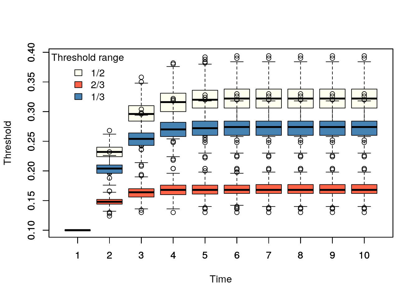
ans_1and3 <-rdiffnet_multiple(# Num of simR = nsim,# Statisticstatistic =function(d) cumulative_adopt_count(d)["prop",], seed.graph = net,t =10,threshold.dist =sample(1:3, 500, TRUE),seed.nodes ="random",seed.p.adopt = .1,rewire =FALSE,exposure.args =list(outgoing=FALSE, normalized=FALSE),# Running on 4 coresncpus =4L )
Given the following types of networks: Small-world, Scale-free, Bernoulli, what set of n initiators maximizes diffusion?
Statistical inference
Moran’s I
Moran’s I tests for spatial autocorrelation.
netdiffuseR implements the test in moran, which is suited for sparse matrices.
We can use Moran’s I as a first look to whether there is something happening: let that be influence or homophily.
Using geodesics
One approach is to use the geodesic (shortest path length) matrix to account for indirect influence.
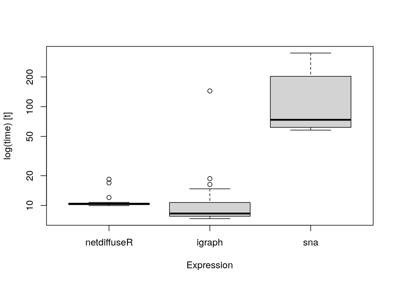
netdiffuseR has a function to do so, the approx_geodesic function, which, using graph powers, computes the shortest path up to n steps. This could be faster (if you only care up to n steps) than igraph or sns:
The summary.diffnet method already runs Moran’s for you. What happens under the hood is:
# For each time point we compute the geodesic distances matrixW <-approx_geodesic(medInnovationsDiffNet$graph[[1]])# We get the element-wise inverseW@x <-1/W@x# And then compute moranmoran(medInnovationsDiffNet$cumadopt[,1], W)
For example, if time of adoption is independent of the structure of the network, then the average threshold level will be independent from the network structure as well.
Another way of looking at this is that the test will allow us to see how probable it is to have this combination of network structure and network threshold (if it is uncommon, then we say that the diffusion model is highly likely)
Example Not random TOA
To use this test, netdiffuseR has the struct_test function.
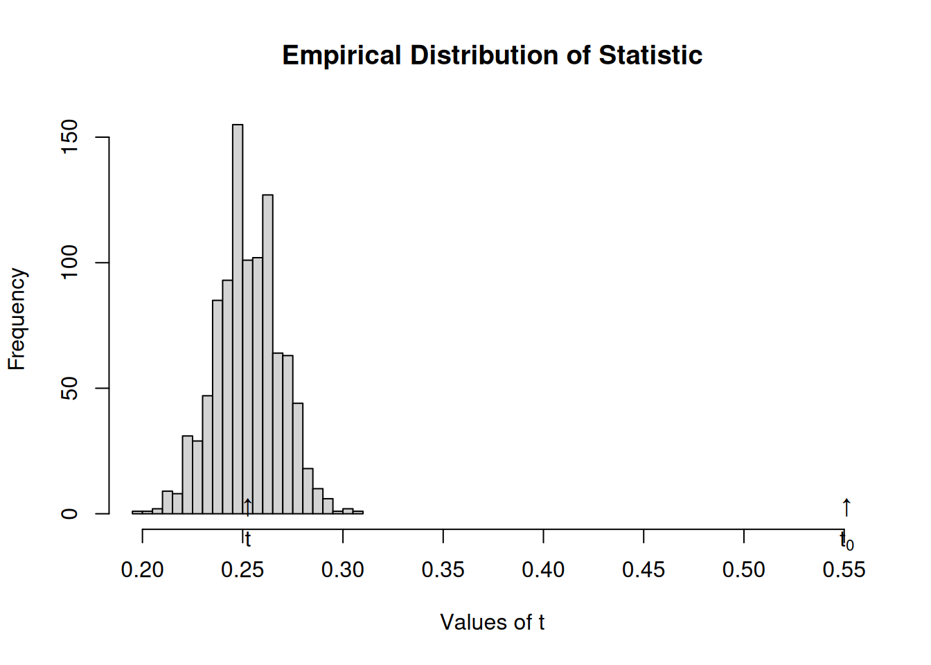
It simulates networks with the same density, and computes a particular statistic every time, generating an EDF (Empirical Distribution Function) under the Null hypothesis (p-values).
# Simulating networkset.seed(1123)net <-rdiffnet(n=500, t=10, seed.graph ="small-world")# Running the testtest <-struct_test(graph = net, statistic =function(x) mean(threshold(x), na.rm =TRUE),R =1e3,ncpus=4, parallel="multicore" )# See the outputtest
Structure dependence test
# Simulations     : 1,000
# nodes           : 500
# of time periods : 10
--------------------------------------------------------------------------------
 H0: E[beta(Y,G)|G] - E[beta(Y,G)] = 0 (no structure dependency)
    observed    expected       p.val
      0.5513      0.2514      0.0000
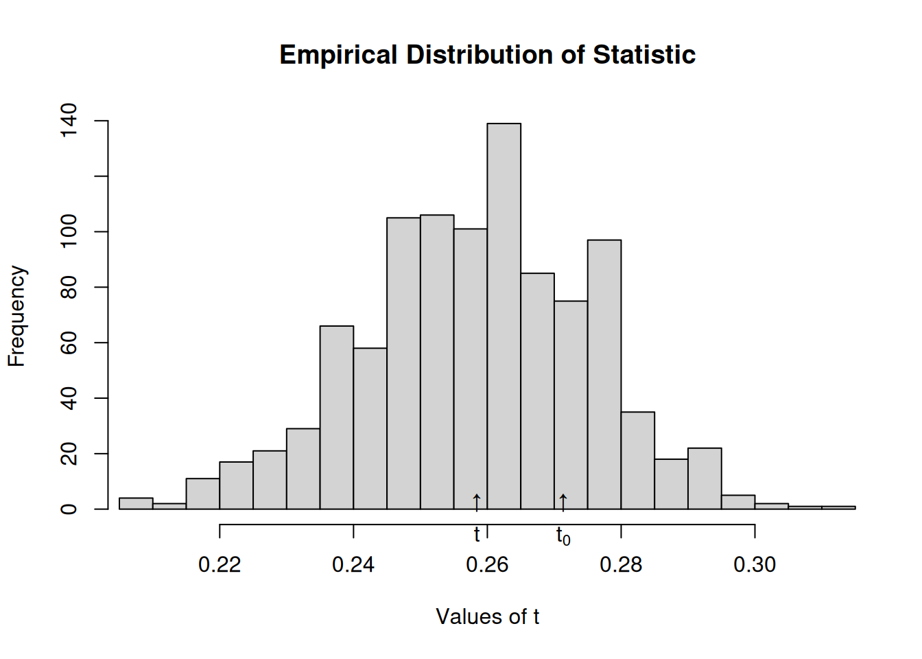
Now we shuffle times of adoption, so that is random
# Resetting TOAs (now will be completely random)diffnet.toa(net) <-sample(diffnet.toa(net), nnodes(net), TRUE)# Running the testtest <-struct_test(graph = net, statistic =function(x) mean(threshold(x), na.rm =TRUE),R =1e3,ncpus=4, parallel="multicore" )# See the outputtest
Structure dependence test
# Simulations     : 1,000
# nodes           : 500
# of time periods : 10
--------------------------------------------------------------------------------
 H0: E[beta(Y,G)|G] - E[beta(Y,G)] = 0 (no structure dependency)
    observed    expected       p.val
      0.2714      0.2585      0.3900
Regression analysis
In regression analysis, we want to see if exposure, once we control for other covariates, had any effect on adopting a behavior.
The big problem is when we have a latent variable that co-determines both network and behavior.
Regression analysis will be generically biased Unless we can control for that variable.
On the other hand, if you can claim that either such variable doesn’t exist or you actually can control for it, then we have two options: lagged exposure models or contemporaneous exposure models. We will focus on the former.
Lagged exposure models
In this type of model, we usually have the following
Compute Moran’s I as the function summary.diffnet does. To do so, you’ll need to use the function toa_mat (which calculates the cumulative adoption matrix), and approx_geodesic (which computes the geodesic matrix). (see ?summary.diffnet for more details).
Read the data as diffnet object, and fit the following logit model adopt = Exposure*\gamma + Measure*\beta + \varepsilon. What happens if you exclude the time-fixed effects?