[1] FALSEEgocentric networks
In egocentric social network analysis (ESNA, for our book,) instead of dealing with a single network, we have as many networks as participants in the study. Egos–the main study subjects–are analyzed from the perspective of their local social network. For a more extended view of ESNA, look at Raffaele Vacca’s “Egocentric network analysis with R”.
In this chapter, I show how to work with one particular type of ESNA data: information generated by the tool Network Canvas. You can download an “artificial” ZIP file containing the outputs from a Network Canvas project here1. We assume the ZIP file was extracted to the folder data-raw/egonets. You can go ahead and extract the ZIP by point-and-click or use the following R code to automate the process:
unzip(
  zipfile = "data-raw/networkCanvasExport-fake.zip",
  exdir   = "data-raw/egonets"
  )
This will extract all the files in networkCanvasExport-fake.zip to the subfolder egonets. Let’s take a look at the first few files:
head(list.files(path = "data-raw/egonets"))
## [1] "I_-59190_BRB9111_attributeList_Person.csv"
## [2] "I_-59190_BRB9111_edgeList_Knows.csv"
## [3] "I_-59190_BRB9111_ego.csv"
## [4] "I_-59190_BRB9111.graphml"
## [5] "I-100BB_00B95-90_attributeList_Person.csv"
## [6] "I-100BB_00B95-90_edgeList_Knows.csv"
As you can see, for each ego in the dataset, there are four files:
...attributeList_Person.csv: Attributes of the alters....edgeList_Knows.csv: Edgelist indicating the ties between the alters....ego.csv: Information about the egos....graphml: And agraphmlfile that contains the egonets.
The next sections will illustrate, file by file, how to read the information into R, apply any required processing, and store the information for later use. We start with the graphml files.
Network files (graphml)
The graphml files can be read directly with igraph’s read_graph function. The key is to take advantage of R’s lists to avoid writing over and over the same block of code, and, instead, manage the data through lists.
Just like any data-reading function, read_graph function requires a file path to the network file. The function we will use to list the required files is list.files():
# We start by loading igraph
library(igraph)

# Listing all the graphml files
graph_files <- list.files(
  path       = "data-raw/egonets", # Where are these files
  pattern    = "*.graphml",        # Specify a pattern for only listing graphml
  full.names = TRUE                # And we make sure we use the full name
                                   # (path.) Otherwise, we would only get names.
  )

# Taking a look at the first three files we got
graph_files[1:3]
## [1] "data-raw/egonets/I_-59190_BRB9111.graphml"
## [2] "data-raw/egonets/I-100BB_00B95-90.graphml"
## [3] "data-raw/egonets/I-1BB79950-0-7.graphml"

# Applying igraph's read_graph
graphs <- lapply(
  X      = graph_files,       # List of files to read
  FUN    = read_graph,        # The function to apply
  format = "graphml"          # Argument passed to read_graph
  )
If the operation succeeded, the previous code block should generate a list of igraph objects named graphs. Let’s take a peek at the first two:
graphs[[1]]
## IGRAPH 1a7b1a4 U--- 12 25 --
## + attr: age (v/n), healthy_diet (v/n), gender_1 (v/l), eat_with_2
## | (v/l), id (v/c)
## + edges from 1a7b1a4:
## [1] 1-- 3 1-- 2 1-- 6 1-- 5 1-- 4 1-- 8 1--11 1--10 2-- 3 3-- 7 3-- 4 3-- 5
## [13] 3-- 6 2-- 7 2-- 4 2-- 5 2-- 6 5-- 6 6--10 7-- 9 4-- 5 5-- 7 4--11 6-- 7
## [25] 4-- 7
graphs[[2]]
## IGRAPH b6a6a05 U--- 16 47 --
## + attr: age (v/n), healthy_diet (v/n), gender_1 (v/l), eat_with_2
## | (v/l), id (v/c)
## + edges from b6a6a05:
## [1] 7--13 1-- 5 1-- 6 1-- 4 1-- 2 7--15 1-- 3 11--13 1--10 1--16
## [11] 4-- 6 2-- 6 6-- 7 1--11 11--15 6-- 9 6-- 8 3-- 9 5--15 4-- 5
## [21] 2-- 5 5-- 8 5-- 7 5--10 3-- 5 6--14 12--13 6--13 3--13 2-- 3
## [31] 3-- 4 3--16 3--11 10--14 7--14 2-- 4 2--10 2--15 10--12 4-- 7
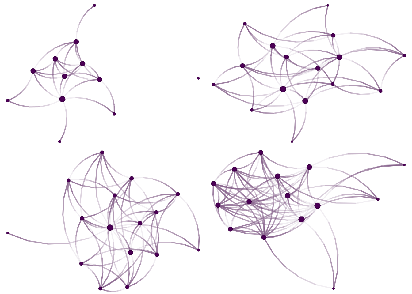
## [41] 6--10 5--11 9--10 1-- 9 1--12 3--12 4--14As always, one of the first things we do with networks is visualize them. We will use the netplot R package (by yours truly) to draw the figures:
library(netplot)
library(gridExtra)

# Graph layout is random
set.seed(1231)

# The grid.arrange allows putting multiple netplot graphs into the same page
grid.arrange(
  nplot(graphs[[1]]),
  nplot(graphs[[2]]),
  nplot(graphs[[3]]),
  nplot(graphs[[4]]),
  ncol = 2, nrow = 2
)
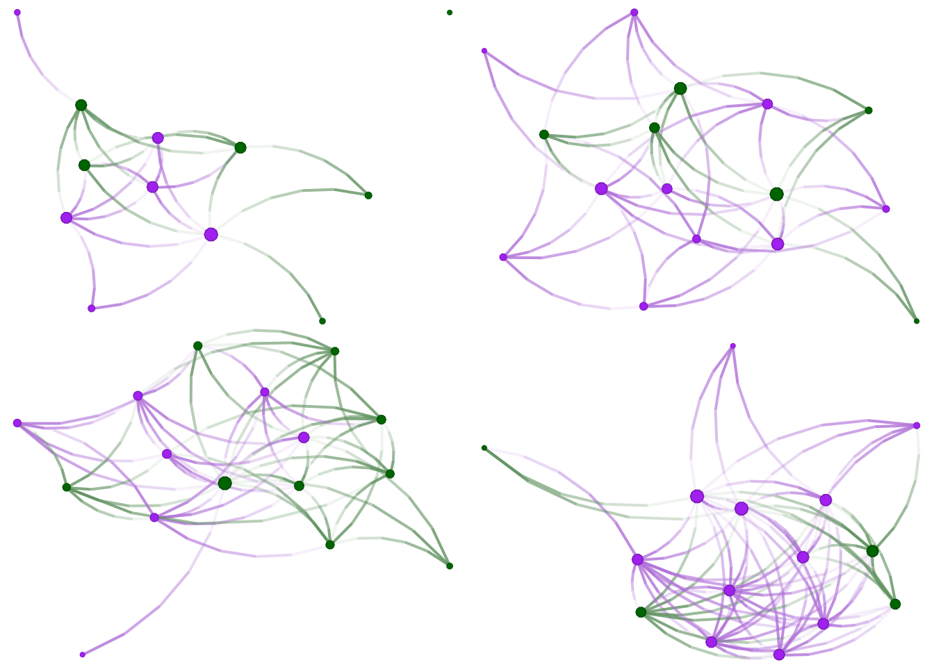
Great! Since nodes in our network have features, we can add a little color. We will use the eat_with_2 variable, coded as TRUE or FALSE. Vertex colors can be specified using the vertex.color argument of the nplot function. In our case, we will specify colors passing a vector with length equal to the number of nodes in the graph. Furthermore, since we will be doing this multiple times, it is worthwhile writing a function:
# A function to color by the eat with variable
color_it <- function(net) {

  # Coding eat_with_2 to be 1 (FALSE) or 2 (TRUE)
  eatswith <- V(net)$eat_with_2

  # Subsetting the color
  ifelse(eatswith, "purple", "darkgreen")

}
This function takes two arguments: a network and a vector of two colors. Vertex attributes in igraph can be accessed through the V(...)$... function. For this example, to access the attribute eat_with_2 in the network net, we type V(net)$eat_with_2. Finally, individuals with eat_with_2 equal to true will be colored purple; otherwise, if equal to FALSE, they will be colored darkgreen. Before plotting the networks, let’s see what we get when we access the eat_with_2 attribute in the first graph:
V(graphs[[1]])$eat_with_2
##  [1]  TRUE  TRUE FALSE FALSE  TRUE  TRUE FALSE FALSE  TRUE  TRUE FALSE FALSE
A logical vector. Now let’s redraw the figures:
grid.arrange(
  nplot(graphs[[1]], vertex.color = color_it(graphs[[1]])),
  nplot(graphs[[2]], vertex.color = color_it(graphs[[2]])),
  nplot(graphs[[3]], vertex.color = color_it(graphs[[3]])),
  nplot(graphs[[4]], vertex.color = color_it(graphs[[4]])),
  ncol = 2, nrow = 2
)
Since most of the time, we will be dealing with many egonets; you may want to draw each network independently; the following code block does that. First, if needed, will create a folder to store the networks. Then, using the lapply function, it will use netplot::nplot() to draw the networks, add a legend, and save the graph as .../graphml_[number].png, where [number] will go from 01 to the total number of networks in graphs.
if (!dir.exists("egonets/figs/egonets"))
  dir.create("egonets/figs/egonets", recursive = TRUE)

lapply(seq_along(graphs), function(i) {

  # Creating the device
  png(sprintf("egonets/figs/egonets/graphml_%02i.png", i))

  # Drawing the plot
  p <- nplot(
    graphs[[i]],
    vertex.color = color_it(graphs[[i]])
    )

  # Adding a legend
  p <- nplot_legend(
    p,
    labels = c("eats with: FALSE", "eats with: TRUE"),
    pch    = 21,
    packgrob.args = list(side = "bottom"),
    gp            = gpar(
      fill = c("darkgreen", "purple")
    ),
    ncol = 2
  )

  print(p)

  # Closing the device
  dev.off()
})
Person files
Like before, we list the files ending in Person.csv (with the full path,) and read them into R. While R has the function read.csv, here I use the function fread from the data.table R package. Alongside dplyr, data.table is one of the most popular data-wrangling tools in R. Besides syntax, the biggest difference between the two is performance; data.table is significantly faster than any other data management package in R, and is a great alternative for handling large datasets. The following code block loads the package, lists the files, and reads them into R.
# Loading data.table
library(data.table)

# Listing the files
person_files <- list.files(
  path       = "data-raw/egonets",
  pattern    = "*Person.csv",
  full.names = TRUE
  )

# Loading all into a single list
persons <- lapply(person_files, fread)

# Looking into the first element
persons[[1]]
##     nodeID   age
##      <int> <int>
##  1:      1    45
##  2:      2    32
##  3:      3    31
##  4:      4    45
##  5:      5    43
##  6:      6    47
##  7:      7    45
##  8:      8    62
##  9:      9    28
## 10:     10    41
## 11:     11    41
## 12:     12    46
## 13:     13    46
## 14:     14    46
## 15:     15    62
## 16:     16    41
A common task is adding an identifier to each dataset in persons so we know from to which ego they belong. Again, the lapply function is our friend:
persons <- lapply(seq_along(persons), function(i) {
  persons[[i]][, dataset_num := i]
})
In data.table, variables are created using the := symbol. The previous code chunk is equivalent to this:
for (i in 1:length(persons)) {
  persons[[i]]$dataset_num <- i
}
If needed, we can transform the list persons into a data.table object (i.e., a single data.frame) using the rbindlist function2. The next code block uses that function to combine the data.tables into a single dataset.
# Combining the datasets
persons <- rbindlist(persons)
persons
##      nodeID   age dataset_num
##       <int> <int>       <int>
##   1:      1    45           1
##   2:      2    32           1
##   3:      3    31           1
##   4:      4    45           1
##   5:      5    43           1
##  ---
## 271:      7    43          19
## 272:      8    48          19
## 273:      9    70          19
## 274:     10    46          19
## 275:     11    50          19
Now that we have a single dataset, we can do some data exploration. For example, we can use the package ggplot2 to draw a histogram of alters’ ages.
# Loading the ggplot2 package
library(ggplot2)

# Histogram of age
ggplot(persons, aes(x = age)) +            # Starting off the plot
  geom_histogram(fill = "purple") +      # Adding a histogram
  labs(x = "Age", y = "Frequency") +       # Changing the x/y axis labels
  labs(title = "Alter's Age Distribution") # Adding a title
## `stat_bin()` using `bins = 30`. Pick better value `binwidth`.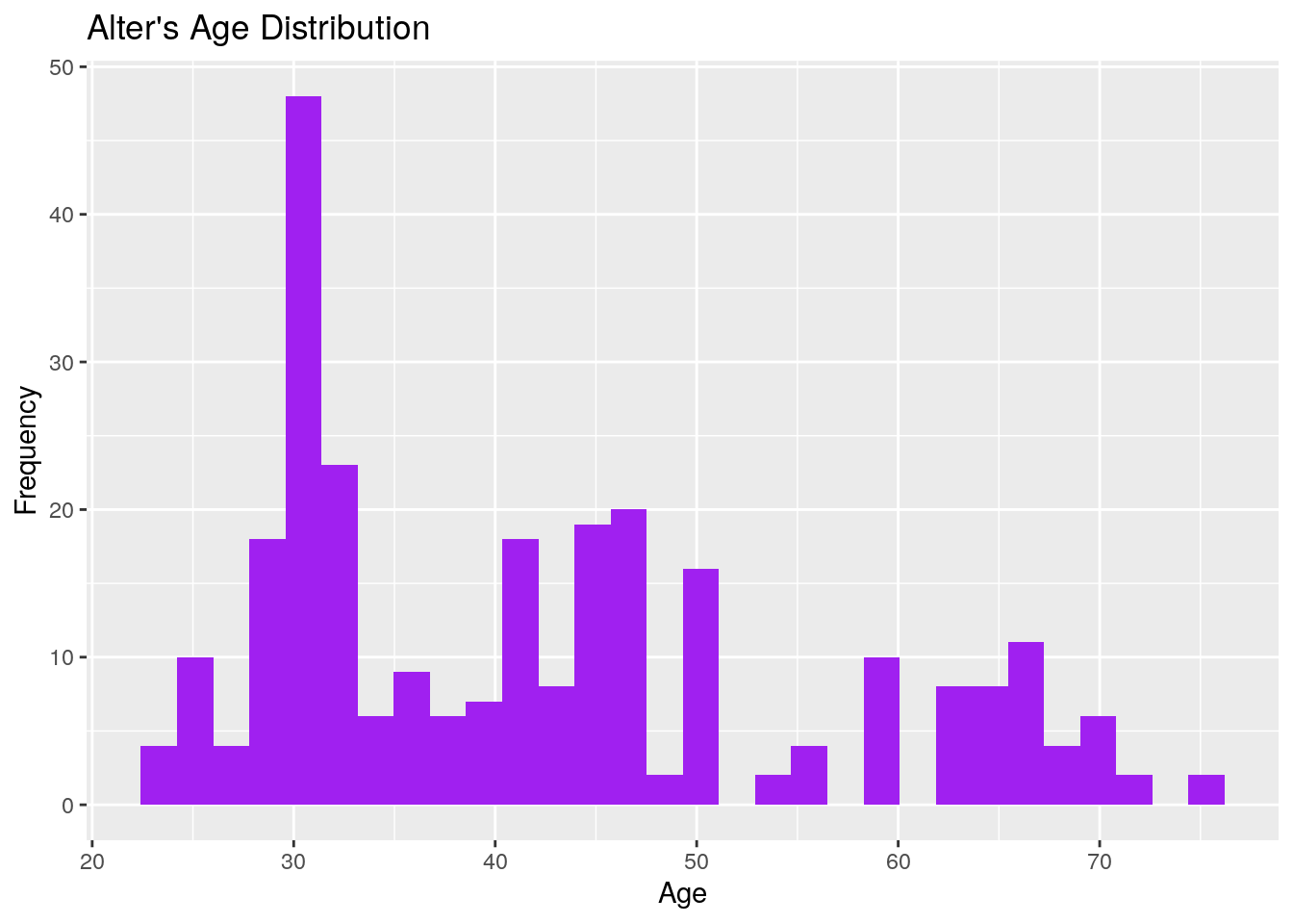
Ego files
The ego files contain information about egos (duh!.) Again, we will read them all at once using list.files + lapply:
# Listing files ending with *ego.csv
ego_files <- list.files(
  path       = "data-raw/egonets",
  pattern    = "*ego.csv",
  full.names = TRUE
  )

# Reading the files with fread
egos <- lapply(ego_files, fread)

# Combining them
egos <- rbindlist(egos)
head(egos)
##                    networkCanvasEgoUUID networkCanvasCaseID
##                                  <char>              <char>
## 1: I-11ca3a78c-62f131f37169-c139217a1f6    I_-59190_BRB9111
## 2: I-fef-ab-4-5a--7-35c4f23-96eb32-34ea    I-100BB_00B95-90
## 3: I2f1bd0b6d-f71f4664cf-d-26-97408f22d      I-1BB79950-0-7
## 4: Id36bb-3b2bcbd2a6239b1103134c6b3d1d6    I000091I_RB010B5
## 5: I436d32fc67fb5c6-23-244f353849b120cd    I019051R0_RRR0-0
## 6: Ibf1f-2-34162bb5f2c36b8241--316a-fff    I01B11-I1101_44R
##                  networkCanvasSessionID
##                                  <char>
## 1: I612b7a1af---0880b-70698204-b-8dbf09
## 2: If5e0-f-26cbec070760f-e6b6d26ebfb06f
## 3: I825c293a1304-e5-cbea8a80aae05b305fa
## 4: I1b8a7d0f6b4-8298c9-848-9186d68a7f3c
## 5: Ie620be37b75983c49ac63-38-425227c959
## 6: Ie3-134323ed40-0e-d954b3d-febbcb9363
##                       networkCanvasProtocolName        sessionStart
##                                          <char>              <POSc>
## 1: Postpartum social networks with sociogram_V5 2023-02-22 23:41:59
## 2: Postpartum social networks with sociogram_V5 2023-02-10 21:46:02
## 3: Postpartum social networks with sociogram_V5 2023-03-01 16:52:09
## 4: Postpartum social networks with sociogram_V5 2023-01-26 20:38:07
## 5: Postpartum social networks with sociogram_V5 2023-02-06 14:55:57
## 6: Postpartum social networks with sociogram_V5 2023-03-16 18:20:02
##          sessionFinish     sessionExported
##                 <POSc>              <POSc>
## 1: 2023-02-23 01:47:00 2023-02-23 01:47:08
## 2: 2023-02-11 01:29:32 2023-02-11 01:34:12
## 3: 2023-03-02 16:51:20 2023-03-02 17:04:42
## 4: 2023-01-26 22:03:20 2023-01-26 22:03:34
## 5: 2023-02-06 15:49:38 2023-02-06 15:56:42
## 6: 2023-03-17 21:11:09 2023-03-17 21:16:15
A cool thing about data.table is that, within square brackets, we can manipulate the data referring to the variables directly. For example, if we wanted to calculate the difference between sessionFinish and sessionStart, using base R we would do the following:
egos$total_time <- egos$sessionFinish - egos$sessionStartWhereas with data.table, variable creation is much more straightforward (notice that instead of using <- or = to assign a variable, we use the := operator):
# How much time?
egos[, total_time := sessionFinish - sessionStart]
We can also visualize this using ggplot2:
ggplot(egos, aes(x = total_time)) +
  geom_histogram() +
  labs(x = "Time in minutes", y = "Count") +
  labs(title = "Total time spent by egos")
## Don't know how to automatically pick scale for object of type <difftime>.
## Defaulting to continuous.
## `stat_bin()` using `bins = 30`. Pick better value `binwidth`.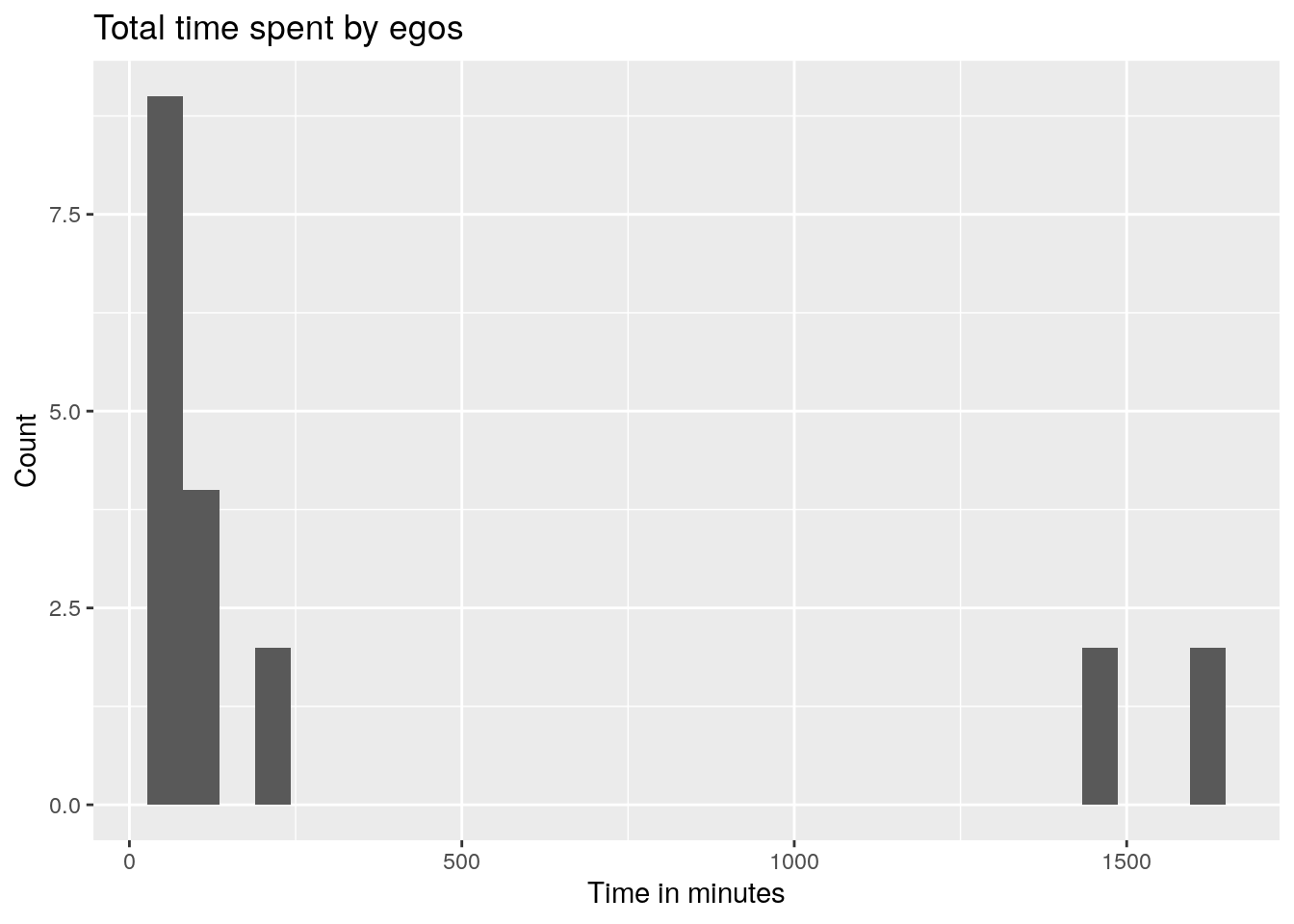
Edgelist files
As I mentioned earlier, since we are reading the graphml files, using the edgelist may not be needed. Nevertheless, the process to import the edgelist file to R is the same we have been applying: list the files and read them all at once using lapply:
# Listing all files ending in Knows.csv
edgelist_files <- list.files(
  path = "data-raw/egonets",
  pattern = "*Knows.csv",
  full.names = TRUE
  )

# Reading all files at once
edgelists <- lapply(edgelist_files, fread)
To avoid confusion, we can also add ids corresponding to the file number. Once we do that, we can combine all files into a single data.table object using rbindlist:
edgelists <- lapply(seq_along(edgelists), function(i) {
  edgelists[[i]][, dataset_num := i]
})

edgelists <- rbindlist(edgelists)

head(edgelists)
##    edgeID  from    to                 networkCanvasEgoUUID
##     <int> <int> <int>                               <char>
## 1:      1     1     5 I839f-8fa8f8aeb8-eaf---ba8-cf3908f3a
## 2:      2     1    10 If81a9c0f-9f4f28ccf-c4c923a-8-0f5fce
## 3:      3     1     9 I899ffe-27-3-a3-ca2fb7f7-ca8e7715ce9
## 4:      4     1    10 I814efaba88cbb02caa8c89790-83beeaf9-
## 5:      5     7     6 Ifd-0eec2e08974eaf2b79f-9efb7e3-8998
## 6:      6     2     6 I-28fe89cc-fc5db3825b92-ae87c-c18e3d
##                       networkCanvasUUID              networkCanvasSourceUUID
##                                  <char>                               <char>
## 1: I720400eb19bccce-77cee773289b02-fe7e I4d5--16a08f8ba463c6458f8979e-65fa9d
## 2: I-b469c0-60f8bbb543-32-628-216f9-038 I-6cf8-f3da-4-96-87efaf5daaa48ba5e5c
## 3: Ifa4933-9baaf5fc-f-e4f5c5e5-ff34-f-f I5-f69a6eaa-5956e8897ca999-ffb6ed-e1
## 4: I4cb-904496b1-6194bcb51b58444b40-ef8 I3e5-6c8d5e0f086--e-5ab45-4-5aaa5-0e
## 5: I0ab7--b7a0ee71e54c1e93cdb-4ca5ab1-b I5-b-9-7eca5ab5-91915ba9b6565a6e42cc
## 6: Ic80142fc4c431009e84b3-ab3f-9b0eab03 Ie0a24eea4e01a4340343a0-66723-a-9970
##                 networkCanvasTargetUUID dataset_num
##                                  <char>       <int>
## 1: Id1c8befd46bdd195c-ce91a8-bc0---4f0e           1
## 2: I757b4a-3ea4d95--b9ebb9db3d55dcbaf-c           1
## 3: I92a62925ff9-e2f27-6ef97d-29fb729624           1
## 4: I7f--da48-46a64-b972c-ef6bbec--64cb4           1
## 5: I-eaa7e95659-9cf01a4f5fd69af54e6-d60           1
## 6: I69060e8a-454609-faa04cd3eeb-5-9550-           1
Putting all together
In this last part of the chapter, we will use the igraph and ergm packages to generate features (covariates, controls, independent variables, or whatever you call them) at the ego-network level. Once again, the lapply function is our friend
Generating statistics using igraph
The igraph R package has multiple high-performing routines to compute graph-level statistics. For now, we will focus on the following statistics: vertex count, edge count, number of isolates, transitivity, and modularity based on betweenness centrality:
net_stats <- lapply(graphs, function(g) {

  # Calculating modularity
  groups <- cluster_edge_betweenness(g)

  # Computing the stats
  data.table(
    size      = vcount(g),
    edges     = ecount(g),
    nisolates = sum(degree(g) == 0),
    transit   = transitivity(g, type = "global"),
    modular   = modularity(groups)
  )
})
Observe we count isolates using the degree() function. We can combine the statistics into a single data.table using the rbindlist function:
net_stats <- rbindlist(net_stats)

head(net_stats)
##     size edges nisolates   transit     modular
##    <num> <num>     <int>     <num>       <num>
## 1:    12    25         1 0.6750000 0.012000000
## 2:    16    47         0 0.4332130 0.003395201
## 3:    16    58         0 0.5612009 0.002675386
## 4:    15    75         0 0.8515112 0.000000000
## 5:    15    52         0 0.5780488 0.000000000
## 6:    17    68         0 0.6291161 0.025735294
Generating statistics based on ergm
The ergm R package has a much larger set of graph-level statistics we can add to our models.3 The key to generating statistics based on the ergm package is the summary_formula function. Before we start using that function, we first need to convert the igraph networks to network objects, which are the native object class for the ergm package. We use the intergraph R package for that, and in particular, the asNetwork function:
# Loading the required packages
library(intergraph)
library(ergm)
## Loading required package: network
##
## 'network' 1.20.0 (2026-02-06), part of the Statnet Project
## * 'news(package="network")' for changes since last version
## * 'citation("network")' for citation information
## * 'https://statnet.org' for help, support, and other information
##
## Attaching package: 'network'
## The following objects are masked from 'package:igraph':
##
##     %c%, %s%, add.edges, add.vertices, delete.edges, delete.vertices,
##     get.edge.attribute, get.edges, get.vertex.attribute, is.bipartite,
##     is.directed, list.edge.attributes, list.vertex.attributes,
##     set.edge.attribute, set.vertex.attribute
##
## 'ergm' 4.11.0 (2025-12-22), part of the Statnet Project
## * 'news(package="ergm")' for changes since last version
## * 'citation("ergm")' for citation information
## * 'https://statnet.org' for help, support, and other information
## 'ergm' 4 is a major update that introduces some backwards-incompatible
## changes. Please type 'news(package="ergm")' for a list of major
## changes.

# Converting all "igraph" objects in graphs to network "objects"
graphs_network <- lapply(graphs, asNetwork)
With the network objects ready, we can proceed to compute graph-level statistics using the summary_formula function. Here we will only look into: the number of triangles, gender homophily, and healthy-diet homophily:
net_stats_ergm <- lapply(graphs_network, function(n) {

  # Computing the statistics
  s <- summary_formula(
    n ~ triangles +
      nodematch("gender_1") +
      nodematch("healthy_diet")
    )

  # Saving them as a data.table object
  data.table(
    triangles       = s[1],
    gender_homoph   = s[2],
    healthyd_homoph = s[3]
  )
})
Once again, we use rbindlist to combine all the network statistics into a single data.table object:
net_stats_ergm <- rbindlist(net_stats_ergm)
head(net_stats_ergm)
##    triangles gender_homoph healthyd_homoph
##        <num>         <num>           <num>
## 1:        27            11               3
## 2:        40            30              20
## 3:        81            40              29
## 4:       216            33              38
## 5:        79            44              19
## 6:       121            38              16
Saving the data
We end the chapter saving all our work into four datasets:
Network statistics (as a csv file)
Igraph objects (as a rda file, which we can read back using
read.rds)Network objects (idem)
Person files (alter’s information, as a csv file.)
CSV files can be saved either using write.csv or, as we do here, fwrite from the data.table package:
# Checking directory exists
if (!dir.exists("data"))
  dir.create("data")

# Network attributes
master <- cbind(egos, net_stats, net_stats_ergm)
fwrite(master, file = "data/network_stats.csv")

# Networks
saveRDS(graphs, file = "data/networks_igraph.rds")
saveRDS(graphs_network, file = "data/networks_network.rds")

# Attributes
fwrite(persons, file = "data/persons.csv")
I thank Jacqueline M. Kent-Marvick, who provided me with what I used as a baseline to generate the artificial Network Canvas export.↩︎
Although not the same,
rbindlist(almost always) yields the same result as calling the functiondo.call. In particular, instead of executing the callrbindlist(persons), we could have useddo.call(rbind, persons).↩︎There’s an obvious reason, ERGMs are all about graph-level statistics!↩︎